plot_forest<-function(data, intercept=TRUE, MA_mean=TRUE){if(MA_mean==FALSE){data<-filter(data, study_id!="overall")}data<-data%>%group_by(study_id)%>%group_nest()%>%hoist(data, "estimate",.remove =FALSE)%>%hoist(estimate, y50 =2)%>%select(-estimate)%>%unnest(data)%>%arrange(y50)%>%mutate(point_shape =case_when(str_detect(type, "summary")~"diamond",TRUE~"circle"))p<-ggplot(data, aes(y =estimate, x =reorder(study_id, y50), ymin =conf.low, ymax =conf.high, shape =point_shape, colour =estimate_type))+geom_pointrange(position =position_jitter(width =0.1))+ggforestplot::theme_forest()+theme(axis.line =element_line(linewidth =0.10, colour ="black"), axis.line.y =element_blank(), text =element_text(family ="Helvetica"))+guides(shape ="none", colour ="none")+coord_flip()+labs(y ="Standardised Out of Sample Predictions, Z", x =element_blank())+scale_y_continuous(breaks =seq(from =round(min(data$conf.low)), to =round(max(data$conf.high)), by =1), minor_breaks =seq(from =-4.5, to =1.5, by =0.5))+NatParksPalettes::scale_color_natparks_d("Glacier")if(intercept==TRUE){p<-p+geom_hline(yintercept =0)}if(MA_mean==TRUE){# p <- p + geom_hline(aes(yintercept = meta_analytic_mean), # data = data,# colour = "#01353D", # linetype = "dashed")}print(p)}plot_forest_2<-function(data, intercept=TRUE, MA_mean=TRUE){if(MA_mean==FALSE){data<-filter(data, study_id!="overall")}plot_data<-data%>%group_by(study_id)%>%group_nest()%>%hoist(data, "estimate",.remove =FALSE)%>%hoist(estimate, y50 =2)%>%select(-estimate)%>%unnest(data)%>%arrange(y50)p<-ggplot(plot_data, aes(y =estimate, x =reorder(study_id, y50), ymin =conf.low, ymax =conf.high,# shape = type, colour =estimate_type))+geom_pointrange(position =position_dodge(width =0.5))+ggforestplot::theme_forest()+theme(axis.line =element_line(linewidth =0.10, colour ="black"), axis.line.y =element_blank(), text =element_text(family ="Helvetica"))+guides(shape ="none", colour ="none")+coord_flip()+labs(y ="Model estimated out of sample predictions", x =element_blank())+scale_y_continuous(breaks =scales::breaks_extended(10))+NatParksPalettes::scale_color_natparks_d("Glacier")if(intercept==TRUE){p<-p+geom_hline(yintercept =0)}if(MA_mean==TRUE){p<-p+geom_hline(aes(yintercept =plot_data%>%filter(type=="summary", estimate_type=="y25")%>%pluck("estimate")), data =data, colour ="#01353D", linetype ="dashed")+geom_hline(aes(yintercept =plot_data%>%filter(type=="summary", estimate_type=="y50")%>%pluck("estimate")), data =data, colour ="#088096", linetype ="dashed")+geom_hline(aes(yintercept =plot_data%>%filter(type=="summary", estimate_type=="y75")%>%pluck("estimate")), data =data, colour ="#58B3C7" , linetype ="dashed")}print(p)}create_model_workflow<-function(outcome, fixed_effects, random_intercepts){# https://community.rstudio.com/t/programmatically-generate-formulas-for-lmer/8575# # ---- roxygen example ----# test_dat <- ManyEcoEvo_results$effects_analysis[[1]] %>%# unnest(review_data) %>%# select(study_id,# starts_with("box_cox_abs_dev"),# RateAnalysis,# PublishableAsIs,# ReviewerId,# box_cox_var)# # test_dat <- test_dat %>%# janitor::clean_names() %>%# mutate_if(is.character, factor) %>%# mutate(weight = importance_weights(1/test_dat$box_cox_var))# create_model_workflow("box_cox_abs_deviation_score_estimate",# "publishable_as_is",# random_intercepts = c("study_id")) %>%# fit(test_dat)# ---- Define random effects constructor function ----randomify<-function(feats){paste0("(1|", feats, ")", collapse =" + ")}# ---- Construct formula ----randomify<-function(feats)paste0("(1|", feats, ")", collapse =" + ")fixed<-paste0(fixed_effects, collapse =" + ")random<-randomify(random_intercepts)model_formula<-as.formula(paste(outcome, "~", fixed, "+", random))# ---- Construct Workflow ----model<-linear_reg()%>%set_engine("lmer")workflow_formula<-workflow()%>%add_variables(outcomes =all_of(outcome), predictors =all_of(c(fixed_effects, random_intercepts)))%>%add_model(model, formula =model_formula)#%>% # add_case_weights(weight)return(workflow_formula)}# Define Plotting Functionplot_model_means_box_cox_cat<-function(dat, variable, predictor_means, new_order, title, back_transform=FALSE){dat<-mutate(dat, "{{variable}}":=# fct_relevel(.f ={{variable}}, new_order))if(back_transform==TRUE){dat<-dat%>%mutate(box_cox_abs_deviation_score_estimate =sae::bxcx(unique(dat$lambda), x =box_cox_abs_deviation_score_estimate, InverseQ =TRUE))predictor_means<-predictor_means%>%as_tibble()%>%mutate(lambda =dat$lambda%>%unique())%>%mutate(across(.cols =-PublishableAsIs,~sae::bxcx(unique(dat$lambda),x =.x, InverseQ =TRUE)))}p<-ggplot(dat, aes(x ={{variable}}, y =box_cox_abs_deviation_score_estimate))+# Add base datgeom_violin(aes(fill ={{variable}}), trim =TRUE, # scale = "count", #TODO consider toggle on/off? colour ="white")+see::geom_jitter2(width =0.05, alpha =0.5)+# Add pointrange and line from meansgeom_line(dat =predictor_means, aes(y =Mean, group =1), linewidth =1)+geom_pointrange( dat =predictor_means,aes(y =Mean, ymin =CI_low, ymax =CI_high), linewidth =1, color ="white", alpha =0.5)+# Improve colorssee::scale_fill_material_d(discrete =TRUE, name ="", palette ="ice", labels =pull(dat, {{variable}})%>%levels()%>%capwords(), reverse =TRUE)+EnvStats::stat_n_text()+see::theme_modern()+theme(axis.text.x =element_text(angle =90))if(back_transform==TRUE){p<-p+labs(x ="Categorical Peer Review Rating", y ="Absolute Deviation from\n Meta-Anaytic Mean Zr")}else{p<-p+labs(x ="Categorical Peer Review Rating", y ="Deviation from\nMeta-Analytic Mean Effect Size")}return(p)}possibly_check_convergence<-possibly(performance::check_convergence, otherwise =NA)possibly_check_singularity<-possibly(performance::check_singularity, otherwise =NA)# define plotting fun for walk plottingplot_continuous_rating<-function(plot_data){plot_data%>%plot_cont_rating_effects(response ="box_cox_abs_deviation_score_estimate", predictor ="RateAnalysis", back_transform =FALSE, plot =FALSE)%>%pluck(2)+ggpubr::theme_pubr()+ggplot2::xlab("Rating")+ggplot2::ylab("Deviation In Effect Size from Analytic Mean")}walk_plot_effects_diversity<-function(model, plot_data, back_transform=FALSE){out_plot<-plot_effects_diversity(model, plot_data, back_transform)+ggpubr::theme_pubr()return(out_plot)}plot_model_means_RE<-function(data, variable, predictor_means){p<-ggplot(data, aes(x =as.factor({{variable}}), y =box_cox_abs_deviation_score_estimate))+# Add base datageom_violin(aes(fill =as.factor({{variable}})), color ="white")+see::geom_jitter2(width =0.05, alpha =0.5)+# Add pointrange and line from meansgeom_line(data =predictor_means, aes(y =Mean, group =1), linewidth =1)+geom_pointrange( data =predictor_means,aes(y =Mean, ymin =CI_low, ymax =CI_high), linewidth =1, color ="white")+# Improve colorsscale_x_discrete(labels =c("0"="No Random Effects", "1"="Random Effects"))+see::scale_fill_material(palette ="ice", discrete =TRUE, labels =c("No Random Effects", "Random effects"), name ="")+see::theme_modern()+EnvStats::stat_n_text()+labs(x ="Random Effects Included", y ="Deviation from meta-analytic mean")+guides(fill =guide_legend(nrow =2))+theme(axis.text.x =element_text(angle =90))return(p)}poss_fit<-possibly(fit, otherwise =NA, quiet =FALSE)create_model_formulas<-function(outcome, fixed_effects, random_intercepts){# https://community.rstudio.com/t/programmatically-generate-formulas-for-lmer/8575# ---- Define random effects constructor function ----randomify<-function(feats){paste0("(1|", feats, ")", collapse =" + ")}# ---- Construct formula ----randomify<-function(feats)paste0("(1|", feats, ")", collapse =" + ")fixed<-paste0(fixed_effects, collapse =" + ")random<-randomify(random_intercepts)model_formula<-as.formula(paste(outcome, "~", fixed, "+", random))return(model_formula)}
C.1 Box-Cox transformation of response variable for model fitting
To aid in interpreting explanatory models where the response variable has been Box-Cox transformed, we plotted the transformation relationship for each of our analysis datasets (Figure C.1). Note that timetk::step_box_cox() directly optimises the estimation of the transformation parameter lambda, \(\lambda\), using the “Guerrero” method such that \(\lambda\) minimises the coefficient of variation for sub-series of a numeric vector (Dancho and Vaughan 2023, see ?timetk::step_box_cox() for further details). Consequently, each dataset has its own unique value of \(\lambda\), and therefore a unique transformation relationship.
During model fitting, especially during fitting of models with random effects using lme4::(Bates et al. 2015), some models failed to converge while others were accompanied with console warnings of singular fit. However, the convergence checks from lme4:: are known to be overly strict (see ?performance::check_convergence() documentation for a discussion of this issue), consequently we checked for model warnings of convergence failure using the performance::check_convergence() function from the performance:: package (Lüdecke et al. 2021). For all models we double-checked that they did not have singular fit by using performance::check_singularity(). Despite passing singularity checks with the performance:: package, parameters::parameters() was unable to properly estimate \(\text{SE}\) and confidence intervals for the random effects of some models, which suggests singular fit. For all models we also checked whether the \(\text{SE}\) of random effects estimates could be calculated, and if not, marked these models as being singular. Analyses of singularity and convergence are presented throughout this document under the relevant section-heading for the analysis type and outcome, i.e. effect size (\(Z_r\)) or out-of-sample predictions (\(y_i\)).
C.3 Deviation Scores as explained by Reviewer Ratings
C.3.1 Effect Sizes \(Z_r\)
Models pf deviation explained by categorical peer ratings all had singular fit or failed to converge for both blue tit and Eucalyptus datasets when random efects were included for both the effect ID and the reviewer ID (Table C.1). For the Eucalyptus dataset, when a random effect was included for effect ID only, the model failed to converge. The same was true for the blue tit dataset. As for the effect-size analysis, we included a random-effect for Reviewer ID only when fitting models of deviation explained by categorical peer ratings (See Table 3.6).
For models of deviation explained by continuous peer-review ratings, when including both random effects for effect ID and Reviewer ID model fits were singular for both datasets (Table C.1). The models passed the performance::check_singularity() check, however, however, the \(\text{SD}\) and CI could not be estimated by parameters::model_parameters() with a warning stating this was likely due to singular fit. For models with a random effect for effect ID, the same occurred for the blue tit dataset, whereas for the Eucalyptus dataset, the model did not converge at all. Consequently, for both blue tit and Euclayptus datasets, we fitted and analysed models of deviation explained by continuous peer review ratings with a random effect for Reviewer ID only (See Table 3.6).
Code
library(multilevelmod)poss_extract_fit_engine<-purrr::possibly(extract_fit_engine, otherwise =NA)poss_parameters<-purrr::possibly(parameters::parameters, otherwise =NA)model<-linear_reg()%>%set_engine("lmer", control =lmerControl(optimizer ="nloptwrap"))base_wf<-workflow()%>%add_model(model)formula_study_id<-workflow()%>%add_variables(outcomes =box_cox_abs_deviation_score_estimate, predictors =c(publishable_as_is, study_id))%>%add_model(model, formula =box_cox_abs_deviation_score_estimate~publishable_as_is+(1|study_id))formula_ReviewerId<-workflow()%>%add_variables(outcomes =box_cox_abs_deviation_score_estimate, predictors =c(publishable_as_is, reviewer_id))%>%add_model(model, formula =box_cox_abs_deviation_score_estimate~publishable_as_is+(1|reviewer_id))formula_both<-workflow()%>%add_variables(outcomes =box_cox_abs_deviation_score_estimate, predictors =c(publishable_as_is, reviewer_id, study_id))%>%add_model(model, formula =box_cox_abs_deviation_score_estimate~publishable_as_is+(1|study_id)+(1|reviewer_id))# ---- Create DF for combinatorial model specification ----model_vars<-bind_rows(tidyr::expand_grid(outcome ="box_cox_abs_deviation_score_estimate", fixed_effects =c("publishable_as_is", "rate_analysis"), random_intercepts =c("study_id", "reviewer_id"))%>%rowwise()%>%mutate(random_intercepts =as.list(random_intercepts)),tidyr::expand_grid(outcome ="box_cox_abs_deviation_score_estimate", fixed_effects =c("publishable_as_is", "rate_analysis"), random_intercepts =c("study_id", "reviewer_id"))%>%group_by(outcome, fixed_effects)%>%reframe(random_intercepts =list(random_intercepts)))# ----- Run all models for all combinations of dataset, exclusion_set, and publishable_subset ----# And Extractset.seed(1234)all_model_fits<-model_vars%>%cross_join(., {ManyEcoEvo::ManyEcoEvo_results%>%select(estimate_type, ends_with("set"), effects_analysis)%>%dplyr::filter(expertise_subset=="All", collinearity_subset=="All")%>%select(-c(expertise_subset, collinearity_subset))})%>%ungroup()%>%filter(publishable_subset=="All", exclusion_set=="complete")%>%select(-c(exclusion_set, publishable_subset))%>%mutate(effects_analysis =map(effects_analysis, ~.x%>%unnest(review_data)%>%select(any_of(c("id_col", "study_id")),starts_with("box_cox_abs_dev"), RateAnalysis, PublishableAsIs,ReviewerId,box_cox_var)%>%janitor::clean_names()%>%mutate_if(is.character, factor)), model_workflows =pmap(.l =list(outcome, fixed_effects, random_intercepts), .f =create_model_workflow), fitted_mod_workflow =map2(model_workflows, effects_analysis, poss_fit), #NOT MEANT TO BE TEST DAT fitted_model =map(fitted_mod_workflow, extract_fit_engine), convergence =map_lgl(fitted_model, performance::check_convergence), singularity =map_lgl(fitted_model, performance::check_singularity), params =map(fitted_model, parameters::parameters))%>%unnest_wider(random_intercepts, names_sep ="_")%>%select(-outcome, -model_workflows, -fitted_mod_workflow,-effects_analysis,estimate_type)%>%replace_na(list(convergence =FALSE))# If singularity == FALSE and convergence == TRUE, but the model appears here, then that's because# the SD and CI's couldn't be estimated by parameters::Zr_singularity_convergence<-all_model_fits%>%left_join({all_model_fits%>%unnest(params)%>%filter(Effects=="random")%>%filter(if_any(contains("SE"), list(is.infinite, is.na)))%>%distinct(fixed_effects, random_intercepts_1,random_intercepts_2, dataset, estimate_type,convergence, singularity)%>%mutate(SE_calc =FALSE)})%>%left_join({all_model_fits%>%unnest(params)%>%filter(Effects=="random")%>%filter(if_any(contains("CI"), list(is.infinite, is.na)))%>%distinct(fixed_effects, random_intercepts_1,random_intercepts_2, dataset, estimate_type,convergence, singularity)%>%mutate(CI_calc =FALSE)})%>%rowwise()%>%mutate(across(ends_with("_calc"), ~replace_na(.x, TRUE)))%>%mutate(across(c(SE_calc, CI_calc, singularity), ~ifelse(is_false(convergence), NA, .x)))# ----- new code showing ALL model fits not just bad fitsZr_singularity_convergence%>%select(-fitted_model, -params, -estimate_type)%>%arrange(dataset,fixed_effects,random_intercepts_1,random_intercepts_2)%>%mutate(across(starts_with("random"), ~str_replace_all(.x, "_", " ")%>%Hmisc::capitalize()%>%str_replace("id", "ID")), dataset =case_when(dataset=="eucalyptus"~Hmisc::capitalize(dataset), TRUE~dataset))%>%group_by(dataset)%>%gt::gt()%>%gt::text_transform( locations =cells_body( columns =fixed_effects, rows =random_intercepts_1!="Reviewer ID"), fn =function(x){paste0("")})%>%tab_style( style =list(cell_fill(color =scales::alpha("red", 0.6)),cell_text(color ="white", weight ="bold")), locations =list(cells_body(columns ="singularity", rows =singularity==TRUE),cells_body(columns ="convergence", rows =convergence==FALSE), #TODO why didn't work here??cells_body(columns ="SE_calc", rows =SE_calc==FALSE),cells_body(columns ="CI_calc", rows =CI_calc==FALSE)))%>%gt::text_transform(fn =function(x)ifelse(x==TRUE, "yes",ifelse(x==FALSE, "no", x)), locations =cells_body(columns =c("singularity", "convergence", "SE_calc", "CI_calc")))%>%gt::opt_stylize(style =6, color ="gray")%>%gt::cols_label(dataset ="Dataset", fixed_effects ="Fixed Effect", singularity ="Singular Fit?", convergence ="Model converged?", SE_calc =gt::md("Can random effects $\\text{SE}$ be calculated?"), CI_calc ="Can random effect 95% CI be calculated?")%>%gt::tab_spanner(label ="Random Effects", columns =gt::starts_with("random"))%>%gt::sub_missing()%>%gt::cols_label_with(columns =gt::starts_with("random"), fn =function(x)paste0(""))%>%gt::tab_style(locations =cells_body(rows =str_detect(dataset, "Eucalyptus"), columns =dataset), style =cell_text(style ="italic"))%>%gt::text_transform(fn =function(x)str_replace(x, "publishable_as_is", "Categorical Peer Rating")%>%str_replace(., "rate_analysis", "Continuous Peer Rating"), locations =cells_body(columns =c("fixed_effects")))%>%gt::tab_style(style =cell_text(style ="italic", transform ="capitalize"), locations =cells_row_groups(groups ="Eucalyptus"))
Table C.1: Singularity and convergence checking outcomes for models of deviation in effect-sizes \(Z_r\) explained by peer-review ratings for different random effect structures. Problematic checking outcomes are highlighted in red.
Fixed Effect
Random Effects
Model converged?
Singular Fit?
Can random effects \(\text{SE}\) be calculated?
Can random effect 95% CI be calculated?
blue tit
Categorical Peer Rating
Reviewer ID
—
yes
no
yes
yes
Study ID
Reviewer ID
yes
no
yes
no
Study ID
—
no
—
—
—
Continuous Peer Rating
Reviewer ID
—
yes
no
yes
yes
Study ID
Reviewer ID
yes
no
no
no
Study ID
—
yes
no
no
no
Eucalyptus
Categorical Peer Rating
Reviewer ID
—
yes
no
yes
yes
Study ID
Reviewer ID
yes
yes
no
no
Study ID
—
no
—
—
—
Continuous Peer Rating
Reviewer ID
—
yes
no
yes
yes
Study ID
Reviewer ID
yes
no
no
no
Study ID
—
no
—
—
—
C.3.2 Out of sample predictions \(y_i\)
As for effect-size estimates \(Z_r\), we encountered convergence and singularity problems when fitting models of deviation in out-of-sample predictions \(y_i\) explained by categorical peer ratings for both datasets (Table C.2). For all continuous models across both datasets, we encountered convergence and singularity problems when including random effects for both effect ID and Reviewer ID, as well as when including random effects for the effect ID only. In the latter case, for many prediction scenarios, across both blue tit and Eucalyptus datasets, estimated random effect coefficient CI’s and \(\text{SE}\) could not be estimated. For models of deviation in out-of-sample predictions explained by continuous peer review ratings, when a random effect was included for effect ID only, CI’s returned values of 0 for both bounds and model means estimated with modelbased::estimate_means() could not be reliably estimated and were equal for every peer-rating category (Table C.2). Consequently, we fitted models of deviation in out-of-sample predictions explained by continuous peer ratings with a random effect for Reviewer ID only (Table C.3). These model structures matched converging and non-singular model structures for effect-size estimates \(Z_r\) (Table C.1).
Table C.2: Singularity and convergence checking outcomes for models of deviation in out-of-sample predictions \(y_r\) explained by peer-review ratings for different random effect structures. Problematic checking outcomes are highlighted in red.
Random Effects
Prediction Scenario
Model converged?
Singular Fit?
Can random effects \(\text{SE}\) be calculated?
Can random effect 95% CI be calculated?
Categorical Peer Rating
Eucalyptus
Reviewer ID
—
$$y_{25}$$
yes
no
yes
yes
Reviewer ID
—
$$y_{50}$$
yes
no
yes
yes
Reviewer ID
—
$$y_{75}$$
yes
yes
no
yes
Eucalyptus
Study ID
Reviewer ID
$$y_{25}$$
yes
no
yes
yes
Study ID
Reviewer ID
$$y_{50}$$
yes
no
yes
yes
Study ID
Reviewer ID
$$y_{75}$$
yes
yes
no
yes
Eucalyptus
Study ID
—
$$y_{25}$$
yes
no
yes
yes
Study ID
—
$$y_{50}$$
yes
no
yes
yes
Study ID
—
$$y_{75}$$
yes
no
yes
yes
blue tit
Reviewer ID
—
$$y_{25}$$
yes
yes
no
yes
Reviewer ID
—
$$y_{50}$$
yes
no
yes
yes
Reviewer ID
—
$$y_{75}$$
yes
no
yes
yes
blue tit
Study ID
Reviewer ID
$$y_{25}$$
yes
no
yes
yes
Study ID
Reviewer ID
$$y_{50}$$
yes
yes
no
yes
Study ID
Reviewer ID
$$y_{75}$$
yes
no
yes
yes
blue tit
Study ID
—
$$y_{25}$$
yes
no
yes
yes
Study ID
—
$$y_{50}$$
yes
no
yes
yes
Study ID
—
$$y_{75}$$
yes
no
yes
yes
Continuous Peer Rating
Eucalyptus
Reviewer ID
—
$$y_{25}$$
yes
no
yes
yes
Reviewer ID
—
$$y_{50}$$
yes
yes
no
yes
Reviewer ID
—
$$y_{75}$$
yes
yes
no
yes
Eucalyptus
Study ID
Reviewer ID
$$y_{25}$$
yes
no
no
yes
Study ID
Reviewer ID
$$y_{50}$$
no
—
—
—
Study ID
Reviewer ID
$$y_{75}$$
yes
no
no
yes
Eucalyptus
Study ID
—
$$y_{25}$$
yes
no
no
yes
Study ID
—
$$y_{50}$$
yes
no
no
yes
Study ID
—
$$y_{75}$$
yes
no
yes
yes
blue tit
Reviewer ID
—
$$y_{25}$$
yes
yes
no
yes
Reviewer ID
—
$$y_{50}$$
yes
no
yes
yes
Reviewer ID
—
$$y_{75}$$
yes
no
yes
yes
blue tit
Study ID
Reviewer ID
$$y_{25}$$
yes
no
no
yes
Study ID
Reviewer ID
$$y_{50}$$
yes
no
no
yes
Study ID
Reviewer ID
$$y_{75}$$
yes
no
no
yes
blue tit
Study ID
—
$$y_{25}$$
yes
no
no
yes
Study ID
—
$$y_{50}$$
yes
no
no
yes
Study ID
—
$$y_{75}$$
yes
no
yes
yes
Code
yi_fitted_mods<-ManyEcoEvo::ManyEcoEvo_yi_viz%>%filter(model_name%in%c("box_cox_rating_cat", "box_cox_rating_cont", "sorensen_glm", "uni_mixed_effects"))%>%select(-ends_with("_plot"), -MA_fit_stats, -contains("mod_"))%>%rowwise()%>%mutate(singularity =possibly_check_singularity(model), convergence =list(possibly_check_convergence(model)))%>%ungroup()%>%mutate(across(where(is.list), .fns =~coalesce(.x, list(NA))))%>%mutate(convergence =list_c(convergence), singularity =case_when(is.na(convergence)~NA,TRUE~singularity))yi_convergence_singularity<-yi_fitted_mods%>%left_join({# Check if SE and CI can be calculatedyi_fitted_mods%>%unnest(model_params)%>%filter(Effects=="random")%>%filter(if_any(contains("SE"), list(is.infinite, is.na)))%>%distinct(dataset, estimate_type, model_name)%>%mutate(SE_calc =FALSE)}, by =join_by(dataset, estimate_type, model_name))%>%left_join({yi_fitted_mods%>%unnest(model_params)%>%filter(Effects=="random")%>%filter(if_any(contains("CI_"), list(is.infinite, is.na)))%>%distinct(dataset, estimate_type, model_name)%>%mutate(CI_calc =FALSE)}, by =join_by(dataset, estimate_type, model_name))%>%rowwise()%>%mutate(across(ends_with("_calc"), ~replace_na(.x, TRUE)),across(c(SE_calc, CI_calc, singularity), ~ifelse(is_false(convergence)|is_na(convergence), NA, .x)), model_name =forcats::as_factor(model_name), model_name =forcats::fct_relevel(model_name, c("box_cox_rating_cat", "box_cox_rating_cont","sorensen_glm","uni_mixed_effects")), model_name =forcats::fct_recode(model_name, `Deviation explained by categorical ratings` ="box_cox_rating_cat", `Deviation explained by continuous ratings` ="box_cox_rating_cont", `Deviation explained by Sorensen's index` ="sorensen_glm", `Deviation explained by inclusion of random effects` ="uni_mixed_effects"), dataset =case_when(str_detect(dataset, "eucalyptus")~"Eucalyptus",TRUE~dataset))%>%ungroup()%>%select(-model)yi_singularity_convergence_sorensen_mixed_mod<-yi_convergence_singularity%>%filter(str_detect(model_name, "Sorensen")|str_detect(model_name, "random"))
We fitted the same deviation models on the out-of-sample-predictions dataset that we fitted for the effect-size dataset. However, while all models of deviation explained by categorical peer-ratings converged, the following datasets and prediction scenarios suffered from singular fit: blue tit - \(y_{25}\), Eucalyptus - \(y_{75}\) (Table C.3). Models of deviation explained by continuous ratings all converged, however models for the out-of-sample predictions model fit was singular. Similarly to the effect-size (\(Z_r\)) dataset, \(\text{SD}\) and CI could not be estimated for random effects in some models (Table C.3), consequently we interpreted this to mean the models had singular fit (See Section C.3.1). Results of all deviation models are therefore presented only for models with non-singular fit, and that converged (Table C.3).
Table C.3: Singularity and convergence checking for models of deviation in out-of-sample-predictions \(y_i\) explained by peer-ratings.
Prediction Scenario
Singular Fit?
Model converged?
Can random effects \(\text{SE}\) be calculated?
Can random effect CI be calculated?
Deviation explained by continuous ratings
blue tit
$$y_{25}$$
yes
yes
no
no
$$y_{50}$$
no
yes
yes
yes
$$y_{75}$$
no
yes
yes
yes
Eucalyptus
$$y_{25}$$
no
yes
yes
yes
$$y_{50}$$
yes
yes
no
no
$$y_{75}$$
yes
yes
no
no
Deviation explained by categorical ratings
blue tit
$$y_{25}$$
yes
yes
no
no
$$y_{50}$$
no
yes
yes
yes
$$y_{75}$$
no
yes
yes
yes
Eucalyptus
$$y_{25}$$
no
yes
yes
yes
$$y_{50}$$
no
yes
yes
yes
$$y_{75}$$
yes
yes
no
no
Group means and \(95\%\) confidence intervals for different categories of peer-review rating are all overlapping (Figure C.2). The fixed effect of peer review rating also explains virtually no variability in deviation scores for out-of-sample predictions \(y_i\) (Table C.3).
Code
yi_violin_cat_plot_data<-ManyEcoEvo::ManyEcoEvo_yi_viz%>%filter(model_name%in%"box_cox_rating_cat")%>%left_join(., {ManyEcoEvo::ManyEcoEvo_yi_results%>%select(dataset, estimate_type, effects_analysis)%>%hoist(effects_analysis, "lambda", .transform =unique)%>%select(-effects_analysis)}, by =join_by(dataset, estimate_type))%>%mutate( dataset =case_when(str_detect(dataset, "eucalyptus")~"Eucalyptus",TRUE~dataset))%>%semi_join({yi_convergence_singularity%>%filter(str_detect(model_name, "categorical"), !singularity, convergence, SE_calc, CI_calc)}, by =join_by("dataset", "estimate_type"))%>%select(dataset, estimate_type, model_name, model)%>%mutate(predictor_means =map(model, modelbased::estimate_means, backend ="marginaleffects"), model_data =map(model, ~pluck(.x, "frame")%>%drop_na()%>%as_tibble()), plot_name =paste(dataset, estimate_type,"violin_cat", sep ="_"))%>%mutate(model_data =map(model_data, .f =~mutate(.x, PublishableAsIs =str_replace(PublishableAsIs,"publishable with ", "")%>%str_replace("deeply flawed and ", "")%>%capwords())), predictor_means =map(predictor_means, .f =~mutate(.x, PublishableAsIs =str_replace(PublishableAsIs,"publishable with ", "")%>%str_replace("deeply flawed and ", "")%>%capwords())))%>%select(-model)yi_violin_cat_plots<-yi_violin_cat_plot_data%>%pmap(.l =list(.$model_data, .$predictor_means, .$plot_name), .f =~plot_model_means_box_cox_cat(..1, PublishableAsIs, ..2, new_order =c("Unpublishable","Major Revision","Minor Revision","Publishable As Is"),..3))%>%purrr::set_names({yi_violin_cat_plot_data%>%pull(plot_name)%>%stringr::str_split("_violin_cat", 2)%>%map_chr(pluck, 1)})subfigcaps_yi_cat<-yi_violin_cat_plot_data%>%mutate(dataset =case_when(dataset=="Eucalyptus"~paste0("*", dataset, "*"), TRUE~Hmisc::capitalize(dataset)))%>%unite(plot_name, dataset, estimate_type, sep =", ")%>%pull(plot_name)fig_cap_yi_deviation_cat_rating<-paste0("Violin plot of Box-Cox transformed deviation from the meta-analytic mean for $y_i$ estimates as a function of categorical peer-review ratings ratings. Note that higher (less negative) values of the deviation score result from greater deviation from the meta-analytic mean. Grey points for each rating group denote model-estimated marginal mean deviation, and error bars denote 95% CI of the estimate. ", subfigcaps_yi_cat%>%paste0(paste0(paste0("**", LETTERS[1:length(subfigcaps_yi_cat)], "**", sep =""), sep =": "), ., collapse =", "), ".")
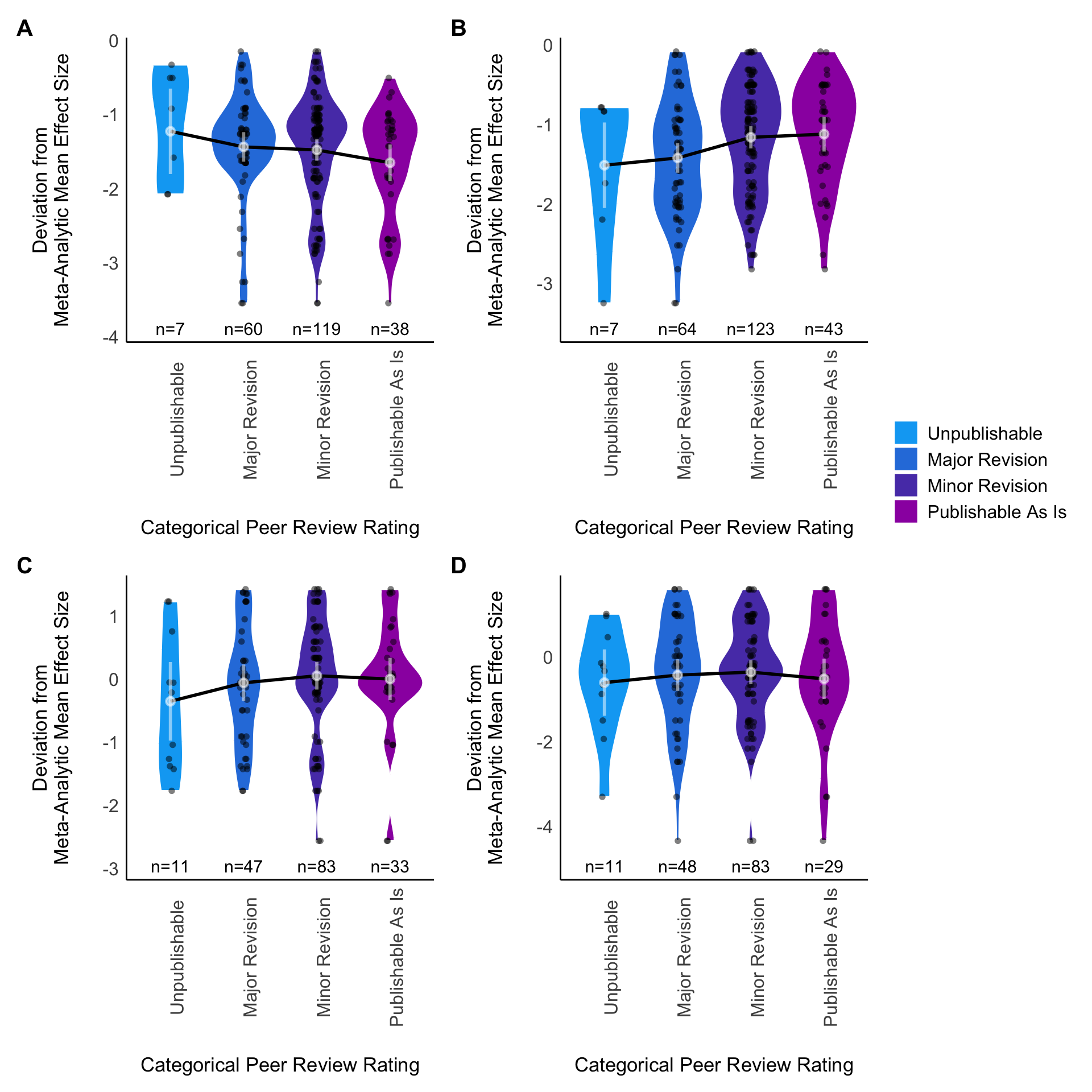
Figure C.2: Violin plot of Box-Cox transformed deviation from the meta-analytic mean for \(y_i\) estimates as a function of categorical peer-review ratings ratings. Note that higher (less negative) values of the deviation score result from greater deviation from the meta-analytic mean. Grey points for each rating group denote model-estimated marginal mean deviation, and error bars denote 95% CI of the estimate. A: Blue tit, y50, B: Blue tit, y75, C: Eucalyptus, y25, D: Eucalyptus, y50.
There was a lack of any clear relationships between quantitative review scores and \(y_i\) deviation scores (Table C.11). Plots of these relationships indicated either no relationship or extremely weak positive relationships (Figure C.3). Recall that positive relationships mean that as review scores became more favorable, the deviation from the meta-analytic mean increased, which is surprising. Because almost no variability in \(y_i\) deviation score was explained by reviewer ratings (Table C.11), this pattern does not appear to merit further consideration.
Code
yi_cont_plot_data<-ManyEcoEvo::ManyEcoEvo_yi_viz%>%filter(model_name%in%c("box_cox_rating_cont"))%>%mutate(dataset =case_match(dataset, "eucalyptus"~"Eucalyptus",.default =dataset))%>%semi_join({yi_convergence_singularity%>%filter(str_detect(model_name, "cont"), # Omit all in-estimable models!singularity, convergence, #SE_calc, #CI_calc)}, by =join_by("dataset", "estimate_type"))%>%select(dataset, estimate_type, model_name, model)%>%mutate(plot_data =map(model, pluck, "frame"))subfigcaps<-yi_cont_plot_data%>%mutate(dataset =case_when(dataset=="Eucalyptus"~paste0("*", dataset, "*"), TRUE~Hmisc::capitalize(dataset)))%>%unite(plot_name, dataset, estimate_type, sep =", ")%>%pull(plot_name)fig_cap_yi_deviation_cont_rating<-paste0("Scatterplots explaining Box-Cox transformed deviation from the meta-analytic mean for $y_i$ estimates as a function of continuous ratings. Note that higher (less negative) values of the deviation score result from greater deviation from the meta-analytic mean. ", subfigcaps%>%paste0(paste0(paste0("**", LETTERS[1:length(subfigcaps)], "**", sep =""), sep =": "), ., collapse =", "), ".")
Figure C.3: Scatterplots explaining Box-Cox transformed deviation from the meta-analytic mean for \(y_i\) estimates as a function of continuous ratings. Note that higher (less negative) values of the deviation score result from greater deviation from the meta-analytic mean. A: Blue tit, y50, B: Blue tit, y75, C: Eucalyptus, y25.
Table C.4: Parameter estimates for univariate models of Box-Cox transformed deviation from the mean \(y_i\) estimate as a function of categorical peer-review rating, continuous peer-review rating, and Sorensen’s index for blue tit and Eucalyptus analyses, and also for the inclusion of random effects for Eucalyptus analyses.
Prediction Scenario
Parameter
Random Effect
Coefficient
\(\text{SE}\)
95%CI
\(t\)
\(\mathit{df}\)
p
Deviation explained by categorical ratings
Eucalyptus
$$y_{25}$$
(Intercept)
−0.35
0.32
[−0.98,0.28]
−1.1
168
0.3
$$y_{25}$$
Publishable with major revision
0.29
0.35
[−0.39,0.98]
0.84
168
0.4
$$y_{25}$$
Publishable with minor revision
0.41
0.34
[−0.26,1.07]
1.21
168
0.2
$$y_{25}$$
Publishable as is
0.35
0.36
[−0.35,1.06]
0.99
168
0.3
$$y_{25}$$
SD (Intercept)
Reviewer ID
0.23
0.15
[0.07,0.79]
$$y_{25}$$
SD (Observations)
Residual
0.92
0.06
[0.82,1.04]
Eucalyptus
$$y_{50}$$
(Intercept)
−0.61
0.4
[−1.4,0.18]
−1.52
165
0.13
$$y_{50}$$
Publishable with major revision
0.18
0.44
[−0.69,1.05]
0.4
165
0.7
$$y_{50}$$
Publishable with minor revision
0.25
0.42
[−0.59,1.09]
0.58
165
0.6
$$y_{50}$$
Publishable as is
0.09
0.47
[−0.83,1.01]
0.19
165
0.8
$$y_{50}$$
SD (Intercept)
Reviewer ID
0.12
0.42
[1.50 × 10−4,1.02 × 102]
$$y_{50}$$
SD (Observations)
Residual
1.29
0.08
[1.14,1.46]
blue tit
$$y_{50}$$
(Intercept)
−1.23
0.29
[−1.81,−0.65]
−4.18
218
<0.001
$$y_{50}$$
Publishable with major revision
−0.21
0.3
[−0.81,0.39]
−0.69
218
0.5
$$y_{50}$$
Publishable with minor revision
−0.25
0.3
[−0.85,0.34]
−0.83
218
0.4
$$y_{50}$$
Publishable as is
−0.42
0.32
[−1.05,0.21]
−1.33
218
0.2
$$y_{50}$$
SD (Intercept)
Reviewer ID
0.22
0.09
[0.11,0.47]
$$y_{50}$$
SD (Observations)
Residual
0.71
0.04
[0.64,0.8]
blue tit
$$y_{75}$$
(Intercept)
−1.51
0.27
[−2.05,−0.97]
−5.52
231
<0.001
$$y_{75}$$
Publishable with major revision
0.09
0.28
[−0.46,0.64]
0.33
231
0.7
$$y_{75}$$
Publishable with minor revision
0.35
0.28
[−0.2,0.9]
1.25
231
0.2
$$y_{75}$$
Publishable as is
0.39
0.29
[−0.19,0.97]
1.33
231
0.2
$$y_{75}$$
SD (Intercept)
Reviewer ID
0.29
0.06
[0.18,0.44]
$$y_{75}$$
SD (Observations)
Residual
0.63
0.03
[0.57,0.7]
Deviation explained by continuous ratings
Eucalyptus
$$y_{25}$$
(Intercept)
−0.46
0.26
[−0.97,0.06]
−1.76
170
0.081
$$y_{25}$$
RateAnalysis
6.14 × 10⁻³
3.54 × 10⁻³
[−8.61 × 10−4,1.31 × 10−2]
1.73
170
0.085
$$y_{25}$$
SD (Intercept)
Reviewer ID
0.12
0.21
[4.27 × 10−3,3.64]
$$y_{25}$$
SD (Observations)
Residual
0.93
0.06
[0.82,1.05]
blue tit
$$y_{50}$$
(Intercept)
−1.35
0.24
[−1.82,−0.88]
−5.65
220
<0.001
$$y_{50}$$
RateAnalysis
−1.82 × 10⁻³
3.05 × 10⁻³
[−7.83 × 10−3,4.18 × 10−3]
−0.6
220
0.6
$$y_{50}$$
SD (Intercept)
Reviewer ID
0.24
0.08
[0.12,0.47]
$$y_{50}$$
SD (Observations)
Residual
0.71
0.04
[0.64,0.79]
blue tit
$$y_{75}$$
(Intercept)
−1.66
0.22
[−2.1,−1.23]
−7.52
233
<0.001
$$y_{75}$$
RateAnalysis
5.62 × 10⁻³
2.79 × 10⁻³
[1.22 × 10−4,1.11 × 10−2]
2.01
233
0.045
$$y_{75}$$
SD (Intercept)
Reviewer ID
0.3
0.06
[0.2,0.45]
$$y_{75}$$
SD (Observations)
Residual
0.63
0.03
[0.57,0.7]
Deviation explained by Sorensen’s index
Eucalyptus
$$y_{25}$$
(Intercept)
−0.3
1.48
[−3.2,2.59]
−0.21
36
0.8
$$y_{25}$$
Mean Sorensen's index
0.44
2.19
[−3.86,4.74]
0.2
36
0.8
Eucalyptus
$$y_{50}$$
(Intercept)
−1.32
2.1
[−5.43,2.79]
−0.63
36
0.5
$$y_{50}$$
Mean Sorensen's index
1.32
3.16
[−4.87,7.51]
0.42
36
0.7
Eucalyptus
$$y_{75}$$
(Intercept)
−0.71
1.78
[−4.19,2.78]
−0.4
36
0.7
$$y_{75}$$
Mean Sorensen's index
0.34
2.71
[−4.96,5.64]
0.12
36
>0.9
blue tit
$$y_{25}$$
(Intercept)
−0.77
0.6
[−1.94,0.4]
−1.29
61
0.2
$$y_{25}$$
Mean Sorensen's index
−0.23
1.04
[−2.27,1.82]
−0.22
61
0.8
blue tit
$$y_{50}$$
(Intercept)
−0.43
0.73
[−1.86,0.99]
−0.6
58
0.6
$$y_{50}$$
Mean Sorensen's index
−1.77
1.27
[−4.26,0.71]
−1.4
58
0.2
blue tit
$$y_{75}$$
(Intercept)
−1.72
0.74
[−3.16,−0.28]
−2.34
61
0.019
$$y_{75}$$
Mean Sorensen's index
0.78
1.28
[−1.73,3.29]
0.61
61
0.5
Deviation explained by inclusion of random effects
Eucalyptus
$$y_{25}$$
(Intercept)
−0.53
0.26
[−1.05,−0.02]
−2.03
36
0.042
$$y_{25}$$
Mixed model
0.74
0.31
[0.13,1.35]
2.37
36
0.018
Eucalyptus
$$y_{50}$$
(Intercept)
−0.57
0.4
[−1.36,0.21]
−1.43
36
0.2
$$y_{50}$$
Mixed model
0.18
0.48
[−0.75,1.11]
0.38
36
0.7
Eucalyptus
$$y_{75}$$
(Intercept)
−0.35
0.39
[−1.11,0.41]
−0.9
36
0.4
$$y_{75}$$
Mixed model
−0.19
0.46
[−1.1,0.71]
−0.41
36
0.7
C.4 Deviation scores as explained by the distinctiveness of variables in each analysis
C.4.1 Out of sample predictions \(y_i\)
Given the convergence and singularity issues encountered with most other analyses, we also checked for convergence and singularity issues in models of deviation explained by Sorensen’s similarity index for \(y_i\) estimates (Table C.5). All models fitted without problem.
Code
yi_sorensen_plot_data<-ManyEcoEvo_yi_viz%>%filter(str_detect(model_name, "sorensen_glm"))%>%mutate( dataset =case_when(str_detect(dataset, "eucalyptus")~"Eucalyptus",TRUE~dataset), model_name =forcats::as_factor(model_name)%>%forcats::fct_relevel(c("box_cox_rating_cat", "box_cox_rating_cont", "sorensen_glm", "uni_mixed_effects"))%>%forcats::fct_recode( `Deviation explained by categorical ratings` ="box_cox_rating_cat", `Deviation explained by continuous ratings` ="box_cox_rating_cont", `Deviation explained by Sorensen's index` ="sorensen_glm", `Deviation explained by inclusion of random effects` ="uni_mixed_effects"))%>%select(dataset, estimate_type, model_name, model)%>%semi_join({yi_convergence_singularity%>%filter(!singularity, convergence, SE_calc, CI_calc)}, by =join_by("dataset", "estimate_type", "model_name"))%>%mutate( plot_data =map(model, ~pluck(.x, "fit", "data")%>%rename(box_cox_abs_deviation_score_estimate =..y)))%>%unite(plot_names, dataset, estimate_type, sep =", ")yi_sorensen_subfigcaps<-yi_sorensen_plot_data$plot_names%>%paste0(paste0(paste0("**", LETTERS[1:length(yi_sorensen_plot_data$plot_names)], "**", sep =""), sep =": "), ., collapse =", ")yi_sorensen_fig_cap<-paste0("Scatter plots examining Box-Cox transformed deviation from the meta-analytic mean for $y_i$ estimates as a function of Sorensen's similarity index. Note that higher (less negative) values of the deviation score result from greater deviation from the meta-analytic mean (@fig-box-cox-transformations). ",yi_sorensen_plot_data$plot_names%>%paste0(paste0(paste0("**", LETTERS[1:length(yi_sorensen_plot_data$plot_names)], "**", sep =""), sep =": "), ., collapse =", "),".")
Figure C.4: Scatter plots examining Box-Cox transformed deviation from the meta-analytic mean for \(y_i\) estimates as a function of Sorensen’s similarity index. Note that higher (less negative) values of the deviation score result from greater deviation from the meta-analytic mean (Figure C.1). A: blue tit, y25, B: blue tit, y50, C: blue tit, y75, D: Eucalyptus, y25, E: Eucalyptus, y50, F: Eucalyptus, y75.
We checked the fitted models for the inclusion of random effects for the Eucalyptus dataset, and for models of deviation explained by Sorensen’s similarity index for \(y_i\) estimates (Table C.5). All models converged, and no singular fits were encountered.
Table C.5: Singularity and convergence checks for models of deviation explained by Sorensen’s similarity index and inclusion of random effects for out-of-sample predictions, \(y_i\). Models of Deviation explained by inclusion of random effects are not presented for blue tit analyses because the number of models not using random effects was less than our preregistered threshold.
Prediction Scenario
Singular Fit?
Model converged?
Can random effects \(\text{SE}\) be calculated?
Can random effects CI be calculated?
Deviation explained by Sorensen's index
blue tit
$$y_{25}$$
no
yes
yes
yes
$$y_{50}$$
no
yes
yes
yes
$$y_{75}$$
no
yes
yes
yes
Eucalyptus
$$y_{25}$$
no
yes
yes
yes
$$y_{50}$$
no
yes
yes
yes
$$y_{75}$$
no
yes
yes
yes
Deviation explained by inclusion of random effects
Eucalyptus
$$y_{25}$$
no
yes
yes
yes
$$y_{50}$$
no
yes
yes
yes
$$y_{75}$$
no
yes
yes
yes
C.5 Deviation scores as explained by the inclusion of random effects
C.5.1 Out of sample predictions \(y_i\)
Only 1 of the Blue tit out-of-sample analyses \(y_i\) included random effects, which was below our preregistered threshold of 5 for running the models of Box-Cox transformed deviation from the meta-analytic mean explained by the inclusion of random-effects. However, 14 Eucalyptus analyses included in the out-of-sample \(y_{i}\) results included only fixed effects, which crossed our pre-registered threshold.
Consequently, we performed this analysis for the Eucalyptus dataset only, here we present results for the out of sample prediction \(y_{i}\) results. There is inconsistent evidence of somewhat higher Box-Cox-transformed deviation values for models including a random effect, meaning the analyses of the Eucalyptus dataset that included random effects averaged slightly higher deviation from the meta-analytic mean out-of-sample estimate in the relevant prediction scenario. This is most evident for the \(y_{25}\) predictions which both shows the greatest difference in Box-Cox transformed deviation values (Figure C.5) and explains the most variation in \(y_i\) deviation score (Table C.4).
Code
yi_deviation_RE_plot_data<-ManyEcoEvo_yi_results%>%mutate(dataset =Hmisc::capitalize(dataset))%>%semi_join({yi_singularity_convergence_sorensen_mixed_mod%>%filter(!singularity, convergence, SE_calc, CI_calc, str_detect(model_name, "random"))}, by =join_by(dataset, estimate_type))%>%select(dataset, estimate_type, model =uni_mixed_effects)%>%rowwise()%>%filter(!is_logical(model))%>%ungroup%>%mutate(predictor_means =map(model, .f =~pluck(.x, "fit")%>%modelbased::estimate_means(.)), plot_data =map(model, pluck, "fit", "data"), plot_data =map(plot_data, rename, box_cox_abs_deviation_score_estimate =..y))%>%mutate(dataset =case_when(str_detect(dataset, "Eucalyptus")~paste0("*", dataset, "*"), TRUE~dataset))%>%unite(plot_names, dataset, estimate_type, sep =", ")yi_deviation_RE_plot_subfigcaps<-yi_deviation_RE_plot_data%>%pull(plot_names)yi_deviation_RE_plot_figcap<-paste0("Violin plot of Box-Cox transformed deviation from meta-analytic mean as a function of presence or absence of random effects in the analyst's model. White points for each rating group denote model-estimated marginal mean deviation, and error bars denote 95% CI of the estimate. Note that higher (less negative) values of Box-Cox transformed deviation result from greater deviation from the meta-analytic mean. ",yi_deviation_RE_plot_data%>%pull(plot_names)%>%paste0(paste0(paste0("**", LETTERS[1:nrow(yi_deviation_RE_plot_data)], "**", sep =""), sep =": "), ., collapse =", "),".")
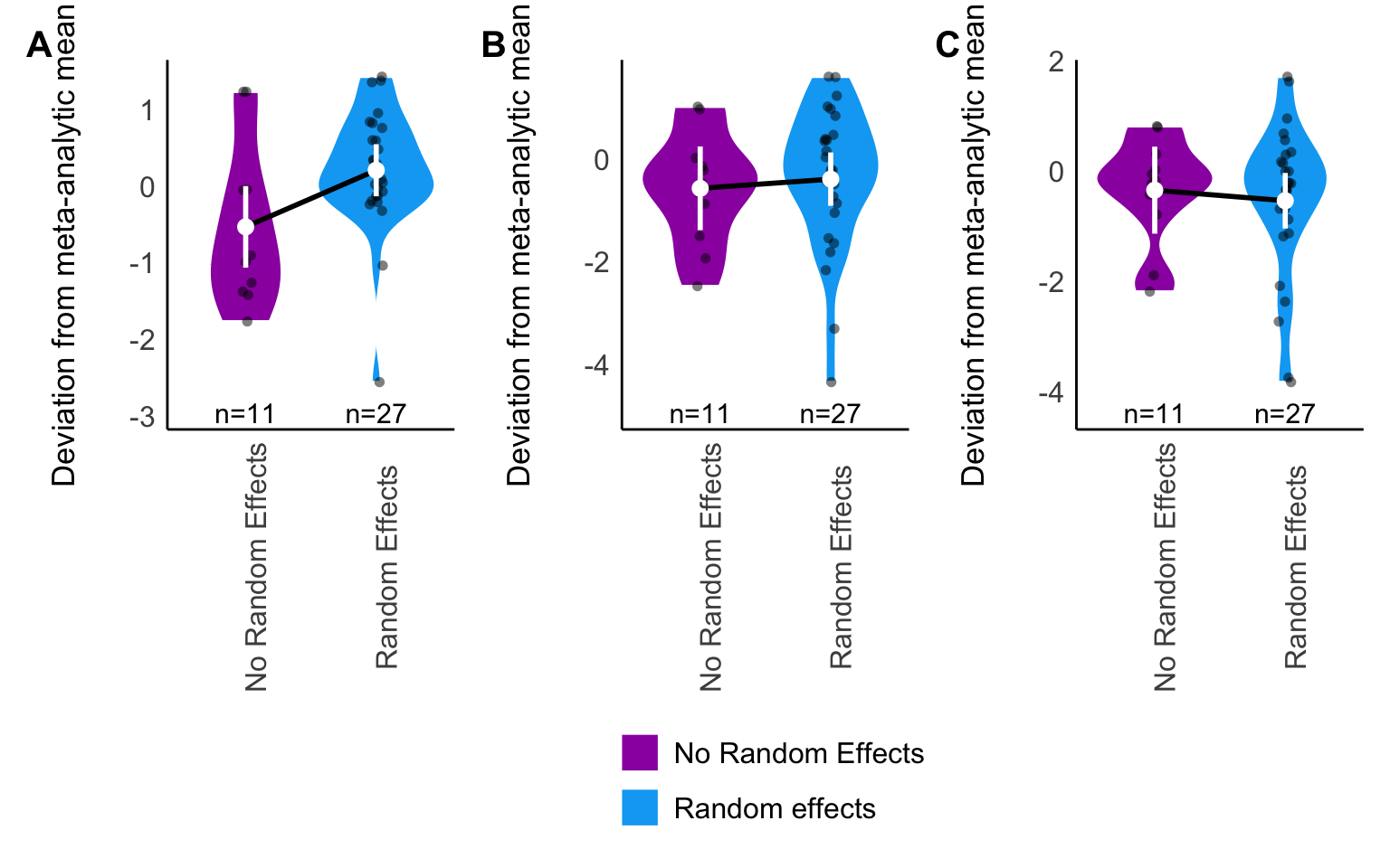
Figure C.5: Violin plot of Box-Cox transformed deviation from meta-analytic mean as a function of presence or absence of random effects in the analyst’s model. White points for each rating group denote model-estimated marginal mean deviation, and error bars denote 95% CI of the estimate. Note that higher (less negative) values of Box-Cox transformed deviation result from greater deviation from the meta-analytic mean. A: Eucalyptus, y25, B: Eucalyptus, y50, C: Eucalyptus, y75.
Table C.6: Parameter estimates from models explaining Box-Cox transformed deviation scores from the mean \(Z_r\) as a function of continuous and categorical peer-review ratings in multivariate analyses. Standard Errors (\(SE\)), 95% confidence intervals (95% CI) are reported for all estimates, while \(\mathit{t}\) values, degrees of freedom (\(\mathit{df}\)) and \(p\)-values are presented for fixed-effects.
Parameter
Random Effect
Coefficient
\(\text{SE}\)
95%CI
t
df
p
blue tit
(Intercept)
−1.24
0.24
[−1.71,−0.77]
−5.16
465
p<0.001
RateAnalysis
−2.84 × 10⁻³
0
[−7.81 × 10−3,2.13 × 10−3]
−1.12
465
p=0.3
Publishable as is
0.06
0.2
[−0.33,0.45]
0.3
465
p=0.8
Publishable with major revision
−0.09
0.14
[−0.36,0.18]
−0.67
465
p=0.5
Publishable with minor revision
−0.02
0.17
[−0.36,0.31]
−0.14
465
p=0.9
Mean Sorensen's index
0.33
0.27
[−0.2,0.87]
1.22
465
p=0.2
SD (Intercept)
Reviewer ID
0.16
0.03
[0.11,0.25]
SD (Observations)
Residual
0.5
0.02
[0.46,0.53]
Eucalyptus
(Intercept)
−2.8
0.77
[−4.32,−1.27]
−3.61
337
p<0.001
RateAnalysis
−0.01
0.01
[−2.27 × 10−2,1.74 × 10−3]
−1.69
337
p=0.093
Publishable as is
0.76
0.54
[−0.3,1.82]
1.42
337
p=0.2
Publishable with major revision
0.65
0.36
[−0.06,1.35]
1.79
337
p=0.074
Publishable with minor revision
0.55
0.44
[−0.32,1.41]
1.24
337
p=0.2
Mean Sorensen's index
0.36
0.91
[−1.43,2.15]
0.39
337
p=0.7
Random included
0.19
0.2
[−0.2,0.59]
0.97
337
p=0.3
SD (Intercept)
Reviewer ID
0.38
0.09
[0.24,0.61]
SD (Observations)
Residual
1.06
0.04
[0.98,1.15]
The multivariate models did a poor job of explaining how different from the meta-analytic mean each analysis would be. For the blue tit analyses the \(R^{2}\) value for the whole model was 0.11 and for the fixed effects component was 0.01, and the residual standard deviation for the model was 0.5. Further, all of the fixed effects had 95% confidence intervals that overlaped 0. This evidence is all consistent with none of the predictor variables in this model (continuous review rating, categorical review rating, distinctiveness of variables included) having any meaningful effect on how far \(Z_r\) estimates fell from the meta-analytic mean for the blue tit analyses. The pattern is largely similar for the Eucalyptus multivariate analysis, in which \(R^{2}\) for the whole model was 0.13 and for the fixed effects component was 0.02, and the residual standard deviation for the model was 1.06. There is somewhat more of a hint of a pattern when examining the parameter estimates from the Eucalyptus analysis. In the case of the fixed effect of categorical reviewer ratings, analyses that were reviewed as ‘publishable as is’ and ‘publishable with major revisions’ appeared to produce results more different from the meta-analytic mean than those that were in the reference class of ‘deeply flawed and unpublishable’. However, the estimates are very uncertain (Eucalyptus fixed effect for ‘publishable as is’ 0.76 (95% CI -0.29,1.81), and for ‘publishable with major revision’ 0.06 (95% CI -0.33,0.45)). Further, the collinearity between the categorical and continuous ratings make interpretation of effects involving either of these two variables unclear, and so we recommend against interpreting the pattern observed here. We report this analysis only for the sake of transparency.
Table C.7: Model summary metrics for multivariate models. \(\sigma\) is the residual standard deviation, ICC is the intra-class correlation coefficient, and \({R}_{M}^2\) and \({R}_{C}^2\) are the marginal and conditional \(R^2\), respectively.
Dataset
\[R^{2}_\text{Conditional}\]
\[R^{2}_\text{Marginal}\]
ICC
RMSE
\[\sigma\]
blue tit
0.11
0.01
0.1
0.48
0.5
Eucalyptus
0.13
0.02
0.11
1.02
1.06
C.6.2 Out of sample predictions \(y_i\)
For the blue tit analyses, the only models that did converge, which were not singular and that had estimable random effect variances were the \(y_{50}\) and \(y_{75}\) prediction scenarios with Reviewer ID as the model random effect (Table C.8). Of the different random effects structures we trialled for the Eucalyptus analyses, only the model that included Reviewer ID as the random effect successfully fitted to the \(y_{50}\) and \(y_{75}\) prediction scenarios, with other models either failing to converge due to complete separation (lme4:: error: Downdated VtV is not positive definite, see https://github.com/lme4/lme4/issues/483).
Code
possibly_parameters<-possibly(parameters::parameters, otherwise =NA)poss_extract_fit_engine<-possibly(extract_fit_engine, otherwise =NA)# ---- Create DF for combinatorial model specification ----model_formulas_multivar<-tidyr::expand_grid(outcome ="box_cox_abs_deviation_score_estimate", random_intercepts =list("study_id", "reviewer_id",c("study_id", "reviewer_id")), fixed_effects =list(c("publishable_as_is", "rate_analysis", "mean_diversity_index", "mixed_model"),c("publishable_as_is", "rate_analysis", "mean_diversity_index")))%>%rowwise()%>%mutate(dataset =case_when(length(fixed_effects)==4~"eucalyptus", TRUE~"blue tit"), wflow_id =paste0("RE:", paste0(random_intercepts, collapse ="_")))%>%unite(wflow_id, dataset, wflow_id, remove =FALSE)%>%rowwise()%>%mutate(model_formulas =list(create_model_formulas(outcome,fixed_effects, random_intercepts))%>%set_names(wflow_id), model_workflows =list(create_model_workflow(outcome, fixed_effects,random_intercepts))%>%set_names(wflow_id))all_model_fits_multivar<-ManyEcoEvo_yi_results%>%select(dataset, estimate_type, effects_analysis)%>%group_by(dataset, estimate_type)%>%nest_join(model_formulas_multivar%>%select(dataset, model_workflows, fixed_effects, random_intercepts), by =join_by(dataset), name ="model_workflow_sets")%>%unnest(model_workflow_sets)%>%rowwise()%>%mutate(effects_analysis =list(effects_analysis%>%select(study_id, starts_with("box_cox_abs_dev"), RateAnalysis, PublishableAsIs,ReviewerId,box_cox_var,mean_diversity_index,mixed_model)%>%janitor::clean_names()%>%mutate_if(is.character, factor)), fitted_mod_workflow =list(poss_fit(model_workflows, effects_analysis)), fitted_model =list(poss_extract_fit_engine(fitted_mod_workflow)), convergence =list(if(!is.na(fitted_model))possibly_check_convergence(fitted_model)), singularity =list(if(!is.na(fitted_model))possibly_check_singularity(fitted_model)), params =list(if(!is.na(fitted_model))possibly_parameters(fitted_model)), fixed_effects =paste0(fixed_effects, collapse =", "))%>%unnest_wider(random_intercepts, names_sep ="_")%>%unnest(c(convergence, singularity))%>%rowwise()%>%replace_na(list(convergence =FALSE))%>%select(-model_workflows, -fitted_mod_workflow, -effects_analysis)yi_multivar_singularity_convergence<-all_model_fits_multivar%>%left_join({all_model_fits_multivar%>%unnest(params)%>%filter(Effects=="random")%>%filter(is.na(SE)|is.infinite(SE))%>%distinct(fixed_effects, random_intercepts_1,random_intercepts_2, dataset, estimate_type)%>%mutate(SE_calc =FALSE)}, by =join_by(dataset, estimate_type, random_intercepts_1,random_intercepts_2, fixed_effects))%>%left_join({all_model_fits_multivar%>%unnest(params)%>%filter(Effects=="random")%>%filter(if_any(contains("CI"), list(is.infinite, is.na)))%>%distinct(fixed_effects, random_intercepts_1,random_intercepts_2, dataset, estimate_type)%>%mutate(CI_calc =FALSE)}, by =join_by(dataset, estimate_type, random_intercepts_1,random_intercepts_2, fixed_effects))%>%rowwise()%>%mutate(across(c(SE_calc, CI_calc), ~ifelse(is.na(.x), TRUE, .x)),across(c(SE_calc, CI_calc, singularity), ~ifelse(is_false(convergence), NA, .x)))# If singularity == FALSE and convergence == TRUE, # but the model appears here, then that's because# the SD and CI's couldn't be estimated by parameters::yi_multivar_singularity_convergence%>%select(-fixed_effects, -fitted_model, -params)%>%arrange(random_intercepts_1,random_intercepts_2, dataset,estimate_type)%>%mutate(across(starts_with("random"), ~str_replace_all(.x, "_", " ")%>%Hmisc::capitalize()%>%str_replace("id", "ID")), dataset =str_replace(dataset, "eucalyptus", "*Eucalyptus*"))%>%group_by(dataset)%>%gt::gt(rowname_col ="estimate_type")%>%tab_style( style =list(cell_fill(color =scales::alpha("red", 0.6)),cell_text(color ="white", weight ="bold")), locations =list(cells_body(columns ="singularity", rows =singularity==TRUE),cells_body(columns ="convergence", rows =convergence==FALSE), #TODO why didn't work here??cells_body(columns ="SE_calc", rows =SE_calc==FALSE),cells_body(columns ="CI_calc", rows =CI_calc==FALSE)))%>%gt::text_transform(fn =function(x)ifelse(x==TRUE, "yes",ifelse(x==FALSE, "no", x)), locations =cells_body(columns =c("singularity", "convergence", "SE_calc","CI_calc")))%>%gt::opt_stylize(style =6, color ="gray")%>%gt::cols_label(dataset ="Dataset", singularity ="Singular Fit?", convergence ="Model converged?", SE_calc =gt::md("Can random effects $\\text{SE}$ be calculated?"), CI_calc ="Can random effect CI be calculated?")%>%gt::tab_spanner(label ="Random Effects", columns =gt::starts_with("random"))%>%gt::sub_missing()%>%gt::cols_label_with(columns =gt::starts_with("random"), fn =function(x)paste0(""))%>%gt::text_transform(fn =function(x)map(x, gt::md), locations =cells_row_groups())%>%gt_fmt_yi(columns ="estimate_type")
Table C.8: Singularity and convergence checks for all combinations of random effects specifications trialled for across subsets of out of sample predictions \(y_i\) from multivariate models.
Random Effects
Model converged?
Singular Fit?
Can random effects \(\text{SE}\) be calculated?
Can random effect CI be calculated?
blue tit
$$y_{25}$$
Reviewer ID
—
yes
yes
no
no
$$y_{50}$$
Reviewer ID
—
yes
no
yes
yes
$$y_{75}$$
Reviewer ID
—
yes
no
yes
yes
$$y_{25}$$
Study ID
Reviewer ID
yes
yes
no
no
$$y_{50}$$
Study ID
Reviewer ID
yes
no
no
no
$$y_{75}$$
Study ID
Reviewer ID
yes
yes
no
no
$$y_{25}$$
Study ID
—
yes
no
no
no
$$y_{50}$$
Study ID
—
yes
no
no
no
Eucalyptus
$$y_{25}$$
Reviewer ID
—
yes
yes
no
no
$$y_{50}$$
Reviewer ID
—
yes
no
yes
yes
$$y_{75}$$
Reviewer ID
—
yes
no
yes
yes
$$y_{25}$$
Study ID
Reviewer ID
yes
no
no
no
$$y_{50}$$
Study ID
Reviewer ID
yes
yes
no
no
$$y_{25}$$
Study ID
—
yes
no
no
no
$$y_{50}$$
Study ID
—
yes
no
no
no
Consequently, we deviated from our intended plan of using random effects for both Effect ID and Reviewer ID, instead using a single random effect for Reviewer ID for the \(y_{50}\) and \(y_{75}\) prediction scenarios for both blue tit and Eucalyptus datasets (Table C.10, Table C.9).
Table C.11: Model summary metrics for models of Box-Cox transformed deviation from the mean \(y_i\) estimate as a function of categorical peer-review rating, continuous peer-review rating, and Sorensen’s index for blue tit and Eucalyptus analyses, and also for the inclusion of random effects for Eucalyptus analyses. Coefficient of determination, \(R^2\), is reported for models of deviation as a function of Sorensen diversity scores and presence of random effects, while \(R^{2}_\text{Conditional}\), \(R^{2}_\text{Marginal}\) and the intra-class correlation (ICC) are reported for models of deviation as explained by peer-review ratings. For all models the residual standard deviation \(\sigma\), root mean squared error (RMSE) were calculated. The number of observations (\(N_{\text{Obs.}}\)) is displayed for reference.
Prediction Scenario
\[N_{\text{Obs.}}\]
RMSE
\[\sigma\]
\[R^2\]
\[R^{2}_\text{Conditional}\]
\[R^{2}_\text{Marginal}\]
ICC
Deviation explained by Sorensen's index
blue tit
$$y_{25}$$
63
0.58
0.59
7.76 × 10⁻⁴
$$y_{50}$$
60
0.72
0.73
0.03
$$y_{75}$$
63
0.71
0.73
5.99 × 10⁻³
Eucalyptus
$$y_{25}$$
38
0.91
0.94
1.13 × 10⁻³
$$y_{50}$$
38
1.29
1.33
4.82 × 10⁻³
$$y_{75}$$
38
1.26
1.29
4.32 × 10⁻⁴
Deviation explained by continuous ratings
blue tit
$$y_{25}$$
237
0.58
0.58
2.48 × 10⁻⁴
$$y_{50}$$
224
0.68
0.71
0.1
1.74 × 10⁻³
0.1
$$y_{75}$$
237
0.59
0.63
0.2
1.86 × 10⁻²
0.18
Eucalyptus
$$y_{25}$$
174
0.92
0.93
0.04
1.79 × 10⁻²
0.02
$$y_{50}$$
171
1.28
1.29
5.75 × 10⁻⁴
$$y_{75}$$
170
1.23
1.24
1.44 × 10⁻⁴
Deviation explained by categorical ratings
blue tit
$$y_{25}$$
237
0.58
0.58
4.35 × 10⁻³
$$y_{50}$$
224
0.68
0.71
0.1
1.3 × 10⁻²
0.09
$$y_{75}$$
237
0.59
0.63
0.2
3.36 × 10⁻²
0.17
Eucalyptus
$$y_{25}$$
174
0.89
0.92
0.07
1.1 × 10⁻²
0.06
$$y_{50}$$
171
1.27
1.29
0.01
3.39 × 10⁻³
9.14 × 10⁻³
$$y_{75}$$
170
1.23
1.25
1.95 × 10⁻³
Deviation explained by inclusion of random effects
Eucalyptus
$$y_{25}$$
38
0.85
0.87
0.14
$$y_{50}$$
38
1.29
1.33
3.91 × 10⁻³
$$y_{75}$$
38
1.26
1.29
4.76 × 10⁻³
C.8 Post-hoc analysis: checking the use of model weights in all models explaining deviation from the meta-analytic mean
As we describe in Note 2.1, for models of deviation from the meta-analytic mean effect-size, we had intended to use the inverse variance of the Box-Cox transformed deviation from the meta-analytic mean as model weights. Unfortunately using our intended weights specification resulted in invalid transformed response variables for some models whereby extreme outliers were weighted more heavily (two orders of magnitude) than other effect sizes, which caused both issues in the estimated model parameters as well as convergence issues, in particular for models analysing the effect of categorical peer-review rating on deviation from the meta-analytic mean.
Model Weight Calculation Details
We intended to use the invariance of the Box-Cox transformed deviation scores as model weights in our models of deviation from the meta-analytic mean. The variance of the Box-Cox transformation scores is calculated using the delta method (Equation C.1).
\(\mu_{\text{folded}}\) is the folded mean of the deviation scores from the mean for effect \(i\),
\(\text{VAR}_\text{folded}\) is the folded variance of the deviation scores from the mean for effect \(i\),
\(\mu\) is the deviation score from the mean for effect \(i\), calculated as the difference between effect size \(i\) and the mean for all effects: \(\bar{Z}_r - Z_{r_i}\),
\(\sigma\) is the square root of the variance of effect \(i\), \(\text{VZ}_r\),
\(\lambda\) is the Box-Cox transformation parameter (Figure C.1), and
\(\boldsymbol{\phi}\) is the standard normal cumulative distribution function.
Which is executed in the function from the the package, illustrated in the following code snippet:
We systematically investigated the impact of using different weighting schemes (no weights, inverse-Box-Cox transformed variance-, and inverse folded variance-, of the absolute deviation scores) on model convergence, singularity and other model checking metrics to aid decision-making about the appropriate weighting scheme and random-effects structure for these models. Given the convergence issues we encountered when using the intended weights, and that the desired random effects structure could not be fitted, we also investigated the impact of using different random-effects structures (effect ID, reviewer ID, or both effect ID and reviewer ID) on model convergence and singularity. For each weighting scheme, we fitted models with each different random effects structure to both the blue tit and Eucalyptus analyst data, and evaluated model convergence, singularity and model performance using the performance::compare_performance function.
Weight investigation code
# Create filter argument expressionsfilter_args=rlang::exprs(exclusion_set=="complete", publishable_subset=="All",expertise_subset=="All",collinearity_subset=="All")# Create function to prepare ratings dataprepare_ratings_data<-function(effects_analysis){data_tbl<-effects_analysis%>%unnest(cols =c(review_data))%>%select(study_id, TeamIdentifier,starts_with("box_cox_"),ReviewerId, PublishableAsIs,# lambda,folded_v_val)%>%ungroup()%>%mutate(PublishableAsIs =forcats::fct_relevel(PublishableAsIs, c("deeply flawed and unpublishable", "publishable with major revision", "publishable with minor revision", "publishable as is")), obs_id =1:n())return(data_tbl)}# Create base model formulatbase_formula<-rlang::new_formula(rlang::expr(box_cox_abs_deviation_score_estimate), rlang::expr(PublishableAsIs))# Create weight functionscalc_inv_bc_var<-rlang::as_function(~1/pull(.x, box_cox_var))calc_inv_folded_v<-rlang::as_function(~1/pull(.x, folded_v_val))no_weights<-NAweight_formulas<-list(no_weights,calc_inv_bc_var,calc_inv_folded_v)%>%purrr::set_names("no_weights","inv_bc_var","inv_folded_v")# Create random effect expressionsRE_rev<-expr((1|ReviewerId))RE_study<-expr((1|study_id))RE_both<-expr(!!RE_rev+!!RE_study)random_expressions<-list(RE_rev,RE_study,RE_both)%>%purrr::set_names("RE_rev","RE_study","RE_both")# Create model fitting wrapper functionlmer_wrap<-function(data_tbl, random_effect, weight_form, ..., env=caller_env()){f<-rlang::new_formula(expr(box_cox_abs_deviation_score_estimate), expr(PublishableAsIs+!!random_effect), env =env)weights<-if(rlang::is_na(weight_form))NULLelseweight_form(data_tbl)rlang::inject(lme4::lmer(!!f, data =data_tbl, weights =weights, ...))}# Fit all modelsall_models<-ManyEcoEvo_results%>%ungroup%>%filter(!!!filter_args)%>%select(dataset, effects_analysis)%>%hoist(.col =effects_analysis,"lambda", .simplify =TRUE, .transform =unique)%>%mutate(model_data =map(effects_analysis, prepare_ratings_data), .keep ="unused")%>%expand_grid(expand_grid(weight_formulas, random_expressions)%>%mutate(weight_forms =names(weight_formulas), random_effect =names(random_expressions))%>%unite("model_spec", weight_forms, random_effect, sep ="."))%>%# hoist("model_data", weights = list("study_id", "box_cox_var", "folded_v_val"),.remove = F) %>% mutate(model =pmap(list(model_data, random_expressions, weight_formulas), lmer_wrap), .keep ="unused")%>%mutate(singularity =map_lgl(model, performance::check_singularity), convergence =map_lgl(model, performance::check_convergence))possibly_estimate_means<-possibly(modelbased::estimate_means, otherwise =NULL)# Extract Parameter Estimatesestimate_means<-all_models%>%filter(singularity==F, convergence==T)%>%reframe(model =set_names(model, model_spec), dataset =dataset, model_spec =model_spec, weights =case_when(!str_detect(model_spec, "no_weights")~"(weights)", .default =NA))%>%rowwise()%>%mutate(weights =modify_if(list(weights), ~is.na(.x), ~NULL), results =list(possibly_estimate_means(model, by ="PublishableAsIs", weights =weights)))%>%ungroup()%>%mutate(results =set_names(results, dataset))%>%drop_na(results)# model means couldn't be estimated due to convergence issues, drop those models# evaluate and compare performance for remaining modelsmodel_comparison_results<-all_models%>%filter(model_spec!="inv_bc_var.RE_study"|dataset!="eucalyptus")%>%#rm nearly unidentifiable modelsemi_join(estimate_means, by =join_by(dataset, model_spec))%>%group_by(dataset)%>%summarise(model =set_names(model, model_spec)%>%list, results =map(model, performance::compare_performance, rank =T), results =set_names(results, unique(dataset)), .groups ="keep")model_means_results<-estimate_means%>%left_join(model_comparison_results%>%select(-model)%>%unnest(results), by =join_by("dataset", "model_spec"=="Name"))%>%mutate(label =paste(dataset, model_spec, sep ="."))%>%arrange(dataset, desc(Performance_Score))%>%select(Performance_Score, dataset, model_spec, results)%>%mutate(label =paste(dataset, model_spec, sep ="."))
C.8.1 Model Weight Investigation Findings
For the blue tit models of deviation influenced by categorical peer-review rating, no models including study ID as a random-effect were able to be properly fitted, across all model weight specifications Table C.12. For Eucalyptus models with either no weights, or inverse folded variance as weights, only models with Reviewer ID as the random-effect fitted properly. While models with either Reviewer ID or Study ID as the random-effect passed singularity and convergence fit-checks, and had estimable parameter means when the Inverse Box-Cox variance was used as a model weight Table C.12.
Table C.12: Singularity and convergence checks for all combinations of model weights and random-effects structure in models of the effect of categorical peer rating on deviation from the analytic mean. For some models, mean estimates of parameter levels for peer-review rating were not able to be estimated.
Model Weight
Random Effects
Singular Fit?
Model converged?
Means Estimable?
blue tit
None
Reviewer ID
no
yes
yes
Study ID
no
no
no
Reviewer ID and Study ID
yes
yes
no
Inverse Box-Cox variance
Reviewer ID
no
yes
yes
Study ID
no
yes
no
Reviewer ID and Study ID
yes
yes
no
Inverse folded variance
Reviewer ID
no
yes
yes
Study ID
no
yes
no
Reviewer ID and Study ID
yes
yes
no
eucalyptus
None
Reviewer ID
no
yes
yes
Study ID
no
no
no
Reviewer ID and Study ID
no
yes
no
Inverse Box-Cox variance
Reviewer ID
no
yes
yes
Study ID
no
yes
yes
Reviewer ID and Study ID
yes
yes
no
Inverse folded variance
Reviewer ID
no
yes
yes
Study ID
no
yes
no
Reviewer ID and Study ID
yes
yes
no
To check that the alternative weighting methods generated sensible parameter estimates, we generated marginal effects plots for all models that passed the convergence and singularity checks where marginal effects were estimable for both blue tit Figure C.7 and Eucalyptus datasets Figure C.6.
Using the inverse Box-Cox transformed variance for model weights resulted in the marginal mean being pulled towards zero for both datasets, however, this was quite extreme for the Eucalyptus dataset Figure C.6A. When the random-effect for study ID is substituted in place of the reviewer ID, the model means seem more fitting to the data, but uncertainty of estimates seemed artificially small Figure C.6B. For this model, marginal means were all equal in both mean estimate and their standard error when the inverse Box-Cox variance was used as a weight with Study ID as the random effect because the model was nearly unidentifiable Table C.13, so we eliminated this specification from further consideration.
Code
modify_plot<-function(p, .y){p+labs(subtitle =as_label(.y), title =NULL, x ="", y ="Box-Cox transformed\nabsolute deviation from\nmeta-analytic mean")+see::theme_lucid()+theme(axis.text.x =element_text(angle =50, hjust =1))}model_means_results%>%filter(dataset=="eucalyptus")%>%arrange(model_spec)%>%pull(results, name =model_spec)%>%map(., plot, at ="PublishableAsIs")%>%map2(., names(.), modify_plot)%>%patchwork::wrap_plots()+patchwork::plot_annotation(tag_levels ='A')
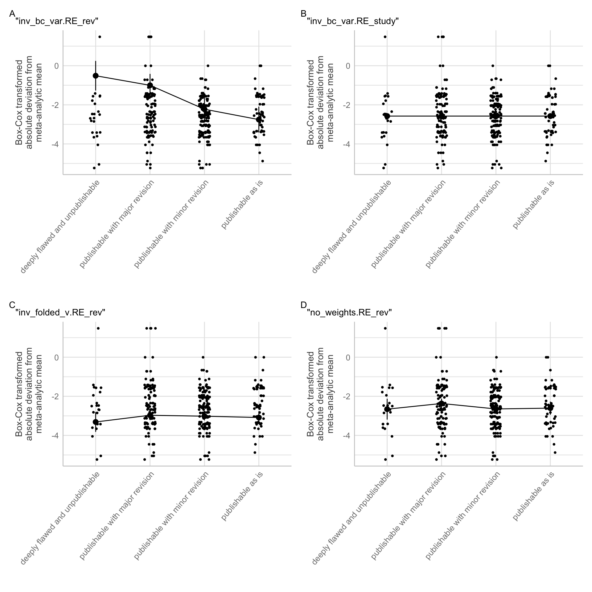
Figure C.6: Effect plots for each non-singular model that converged with estimable fixed effect group means for the Eucalyptus dataset.
Code
modify_plot<-function(p, .y){p+labs(subtitle =as_label(.y), title =NULL, x ="", y ="Box-Cox transformed\nabsolute deviation from\nmeta-analytic mean")+see::theme_lucid()+theme(axis.text.x =element_text(angle =50, hjust =1))}model_means_results%>%filter(dataset=="blue tit")%>%pull(results, name =model_spec)%>%map(., plot, at ="PublishableAsIs")%>%map2(., names(.), modify_plot)%>%patchwork::wrap_plots()+patchwork::plot_annotation(tag_levels ='A')
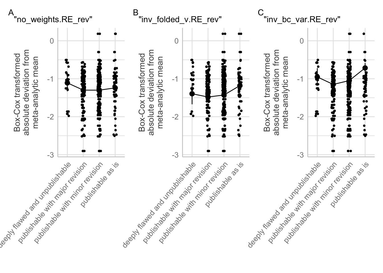
Figure C.7: Effect plots for each non-singular model that converged with estimable fixed effect group means for the blue tit dataset.
Table C.13: Marginal means estimate across weight and random effects specifications for all estimable models for both Eucalyptus and blue tit datasets.
Model Weight
Random Effects
Peer Rating
Mean
\(\text{SE}\)
95%CI
blue tit
None
Reviewer ID
deeply flawed and unpublishable
−1.11
0.11
[−1.33,−0.89]
publishable with major revision
−1.30
0.05
[−1.39,−1.21]
publishable with minor revision
−1.30
0.04
[−1.38,−1.22]
publishable as is
−1.24
0.07
[−1.38,−1.10]
Inverse folded variance
Reviewer ID
deeply flawed and unpublishable
−1.40
0.14
[−1.67,−1.12]
publishable with major revision
−1.48
0.06
[−1.61,−1.35]
publishable with minor revision
−1.43
0.05
[−1.53,−1.32]
publishable as is
−1.18
0.08
[−1.35,−1.01]
Inverse Box-Cox variance
Reviewer ID
deeply flawed and unpublishable
−0.95
0.12
[−1.18,−0.72]
publishable with major revision
−1.15
0.06
[−1.26,−1.03]
publishable with minor revision
−1.05
0.05
[−1.15,−0.95]
publishable as is
−0.72
0.07
[−0.85,−0.58]
eucalyptus
None
Reviewer ID
deeply flawed and unpublishable
−2.66
0.27
[−3.19,−2.12]
publishable with major revision
−2.37
0.12
[−2.61,−2.12]
publishable with minor revision
−2.65
0.11
[−2.86,−2.43]
publishable as is
−2.60
0.17
[−2.94,−2.27]
Inverse folded variance
Reviewer ID
deeply flawed and unpublishable
−3.31
0.26
[−3.82,−2.81]
publishable with major revision
−2.97
0.13
[−3.21,−2.72]
publishable with minor revision
−3.02
0.11
[−3.23,−2.80]
publishable as is
−3.08
0.16
[−3.40,−2.77]
Inverse Box-Cox variance
Reviewer ID
deeply flawed and unpublishable
−0.51
0.39
[−1.27,0.24]
publishable with major revision
−1.00
0.30
[−1.59,−0.42]
publishable with minor revision
−2.22
0.30
[−2.81,−1.64]
publishable as is
−2.76
0.34
[−3.42,−2.09]
Inverse Box-Cox variance
Study ID
deeply flawed and unpublishable
−2.58
0.06
[−2.70,−2.45]
publishable with major revision
−2.58
0.06
[−2.70,−2.45]
publishable with minor revision
−2.58
0.06
[−2.70,−2.45]
publishable as is
−2.58
0.06
[−2.70,−2.45]
After discarding models based on the above criteria, we were left with a subset of models that passed convergence and singularity checks, and had estimable parameter means, all of which included reviewer ID as the only random effect. Although it seemed that the inverse Box-Cox variance resulted skewed estimated marginal means, it was unclear whether the inverse folded variance was a better alternative over using no weights, as the inverse folded variance seemed to exhibit a similar pattern in pulling the estimated marginal effects towards zero, but to a lesser extent than for the inverse Box-Cox variance.
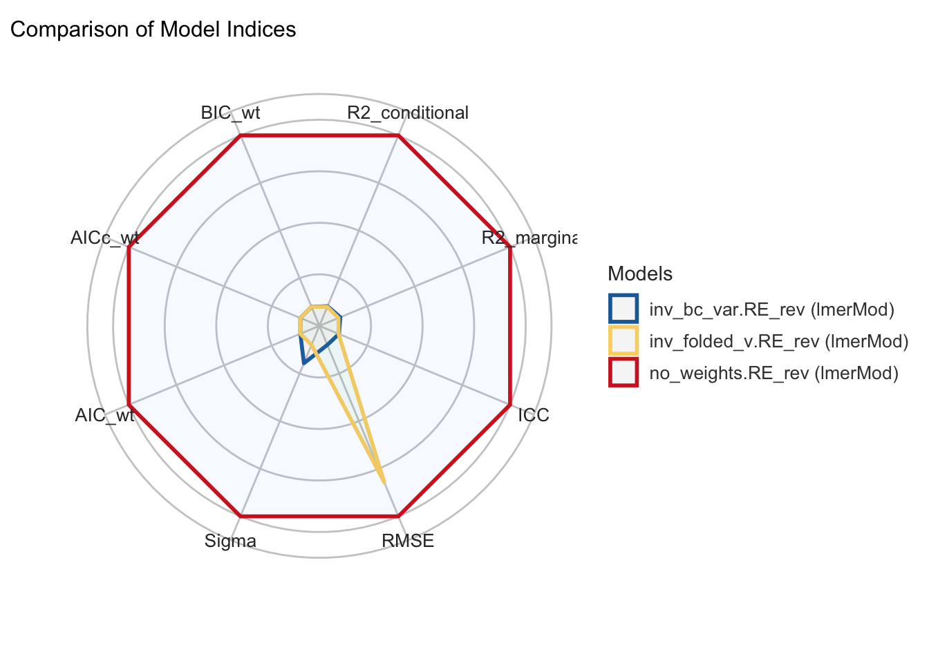
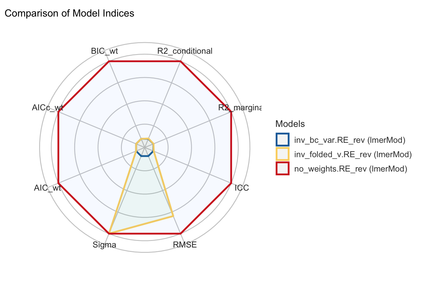
To further aid in decision-making about which model weights to use, we compared the performance of all models that passed the convergence and singularity checks, and had estimable parameter means. We used the performance::compare_performance function to calculate performance metrics for this subset of models, and plotted the results using the performance package’s in-built plotting method, which creates spider plots of normalised performance metrics for each model Figure C.8. For completeness, all model performance results of this final subset are reported in Table C.14.
The performance comparison plots confirmed our suspicions that the inverse Box-Cox variance was not a suitable weight for these models, and it performed relatively poorly across all metrics for both the Eucalyptus and blue tit datasets Figure C.8. The inverse folded variance weighted models performed similarly poorly for both datasets across all metrics except for RMSE in the case of the blue tit dataset, and both Sigma and RMSE for the Eucalyptus dataset. For both datasets using no weights when there is only a random-effect for Reviewer ID resulted in the best model fit and performance across all metrics. In keeping with our informed preference of using no weights, model comparison analysis highlighted that using no weights in the models was preferable.
Code
# plot performance for remaining modelsmodel_comparison_plots<-model_comparison_results%>%mutate(dataset =str_replace(dataset, "eucalyptus", "*Eucalyptus*"))%>%pull(results, "dataset")%>%map(plot)# for printing plot name on figure# model_comparison_plots %>% # map2(.x = ., .y = names(.), ~ .x + ggtitle(.y) #+ # theme(title = ggtext::element_markdown())# )model_comparison_plots
(a) Blue tit models.
(b) Eucalyptus models.
Figure C.8: Model performance comparison plots for a subset of models that passed convergence and singularity checks and had estimable marginal effects. Models are compared based on their performance metrics, including \(R^{2}_\text{Conditional}\), \(R^{2}_\text{Marginal}\), Intra-Class Correlation, Root Mean Squared Error (RMSE), and the weighted AIC, corrected AIC and BIC. Values of performance are normalised across models for each metric, against the top-most performing model across all metrics. Greater distance from the centre on each metric axis indicates dominance in performance. For both blue tit and Eucalyptus models, all included a random effect for Reviewer ID, and weights consisted of the inverse Box-Cox variance for weights (blue line), inverse folded variance (yellow line), or none (red line).
Table C.14: Model performance metric values (non-normalised) for final subset of models considered in weights analysis. All models in final subset included random-effect of Reviewer ID. Metrics included \(R^{2}_\text{Conditional}\), \(R^{2}_\text{Marginal}\), Intra-Class Correlation, Root Mean Squared Error (RMSE), and the weighted AIC, corrected AIC and BIC.
Model Weight
\[AIC\]
\[AIC\] (wt)
\[AIC_c\]
\[AIC_c\] (wt)
\[BIC\]
\[BIC\] (wt)
\[R^{2}_\text{Conditional}\]
\[R^{2}_\text{Marginal}\]
ICC
RMSE
\[\sigma\]
blue tit
None
723.15
1
723.33
1
748.1
1
0.09
7.47 × 10⁻³
0.08
0.4827981
0.5
Inverse Box-Cox variance
840.52
3.26 × 10⁻²⁶
840.7
3.26 × 10⁻²⁶
865.48
3.26 × 10⁻²⁶
7.67 × 10⁻⁴
1.31 × 10⁻⁴
6.36 × 10⁻⁴
0.5822505
11.83
Inverse folded variance
1,026.75
1.19 × 10−66
1,026.93
1.19 × 10−66
1,051.7
1.19 × 10−66
4.71 × 10⁻⁴
5.14 × 10⁻⁵
4.2 × 10⁻⁴
0.5026704
13.19
eucalyptus
None
1,063.74
1
1,063.99
1
1,086.82
1
0.13
0.01
0.12
1.0173409
1.06
Inverse Box-Cox variance
1,386.88
6.80 × 10−71
1,387.12
6.80 × 10−71
1,409.96
6.80 × 10−71
2.28 × 10⁻⁹
2.47 × 10⁻¹⁰
2.03 × 10⁻⁹
1.4993872
4.68 × 10⁴
Inverse folded variance
1,109.35
1.25 × 10⁻¹⁰
1,109.6
1.25 × 10⁻¹⁰
1,132.43
1.25 × 10⁻¹⁰
5.66 × 10⁻⁴
1.82 × 10⁻⁵
5.48 × 10⁻⁴
1.1266586
19.68
Bates, Douglas, Martin Mächler, Ben Bolker, and Steve Walker. 2015. “Fitting Linear Mixed-Effects Models Using lme4.”2015 67 (1): 48. https://doi.org/10.18637/jss.v067.i01.
Lüdecke, Daniel, Mattan S. Ben-Shachar, Indrajeet Patil, Philip Waggoner, and Dominique Makowski. 2021. “performance: An R Package for Assessment, Comparison and Testing of Statistical Models.”Journal of Open Source Software 6 (60): 3139. https://doi.org/10.21105/joss.03139.