As described in the summary statistics section of the manuscript, 63 teams submitted 131 \(Z_r\) model estimates and 43 teams submitted 64 \(y_i\) predictions for the blue tit dataset. Similarly, 40 submitted 79 \(Z_r\) model estimates and 14 teams submitted 24 \(y_i\) predictions for the Eucalytpus dataset. The majority of the blue tit analyses specified normal error distributions and were non-Bayesian mixed effects models. Analyses of the Eucalyptus dataset rarely specified normal error distributions, likely because the response variable was in the form of counts. Mixed effects models were also common for Eucalytpus analyses (Table A.1).
Table A.1: Summary of the number of analysis teams, total analyses, models with normal error distributions, mixed effects models, and models developed with Bayesian statistical methods for effect size analyses only (\(Z_r\)) and out-of-sample prediction only (\(y_i\)).
No. Analyses
No. Teams
Normal Distribution
Mixed Effect
Bayesian
blue tit
$$Z_r$$
131
63
124
128
10
$$y_i$$
64
43
59
63
10
Eucalyptus
$$Z_r$$
79
40
15
62
5
$$y_i$$
24
14
1
16
3
A.1.2 Model composition
The composition of models varied substantially (Table A.2) in regards to the number of fixed and random effects, interaction terms and the number of data points used. For the blue tit dataset, models used up to 19 fixed effects, 12 random effects, and 10 interaction terms and had sample sizes ranging from 76 to 3720. For the Eucalyptus dataset models had up to 13 fixed effects, 4 random effects, 5 interaction terms and sample sizes ranging from 18 to 351.
Table A.2: Mean, standard deviation and range of number of fixed and random variables, interaction terms used in models and analysis sample size (N). Repeated for effect-size analyses only (\(Z_r\)) and out-of-sample predictions only (\(y_i\)).
mean
SD
min
max
Blue tit
Eucalyptus
Blue tit
Eucalyptus
Blue tit
Eucalyptus
Blue tit
Eucalyptus
fixed
$$Z_r$$
5.20
5.01
2.92
3.83
1
1
19
13
$$y_i$$
4.78
4.67
2.35
3.45
1
1
10
13
random
$$Z_r$$
3.53
1.41
2.08
1.09
0
0
10
4
$$y_i$$
4.42
0.96
2.78
0.81
1
0
12
3
interactions
$$Z_r$$
0.44
0.16
1.11
0.65
0
0
10
5
$$y_i$$
0.28
0.17
0.63
0.48
0
0
3
2
N
$$Z_r$$
2611.09
298.43
937.48
106.25
76
18
3720
351
$$y_i$$
2816.71
325.55
773.21
64.17
396
90
3720
350
A.1.3 Choice of variables
The choice of variables also differed substantially among analyses (Table A.3) and some analysts constructed new variables that transformed or aggregated one or more existing variables. The blue tit dataset had a total of 52 candidate variables. These variables were included in a mean of 20.5 \(Z_r\) analyses (range 0- 100). The Eucalyptus dataset had a total of 59 candidate variables. The variables in the Eucalyptus dataset were included in a mean of 8.92 \(Z_r\) analyses (range 0-55).
Code
#table 3 - summary of mean, sd and range for the number of analyses in which each variable was usedTable3%>%rename(SD =sd, subset =subset_name)%>%pivot_wider( names_from =dataset, names_sep =".", values_from =c(mean, SD, min, max))%>%ungroup%>%gt::gt(rowname_col ="subset")%>%gt::tab_spanner_delim(delim =".")%>%gt::fmt_scientific(columns ="mean.blue tit", rows =`mean.blue tit`<0.01, decimals =2)%>%gt::fmt_scientific(columns ="SD.blue tit", rows =`SD.blue tit`<0.01, decimals =2)%>%gt::fmt_scientific(columns ="mean.eucalyptus", rows =`mean.eucalyptus`<0.01, decimals =2)%>%gt::fmt_scientific(columns ="SD.eucalyptus", rows =`SD.eucalyptus`<0.01, decimals =2)%>%gt::fmt_number(decimals =2,drop_trailing_zeros =T, drop_trailing_dec_mark =T)%>%gt::cols_label_with(fn =Hmisc::capitalize)%>%gt::cols_label_with(c(contains("Eucalyptus")), fn =~gt::md(paste0("*",.x, "*")))%>%gt::sub_values(columns =subset, values =c("effects"), replacement =gt::md("$$Z_r$$"))%>%gt::sub_values(columns =subset, values =c("predictions"), replacement =gt::md("$$y_i$$"))%>%gt::sub_values(columns =subset, values =c("all"), replacement =gt::md("All analyses"))%>%gt::opt_stylize(style =6, color ="gray")%>%gt::tab_style( style =gt::cell_text(transform ="capitalize"), locations =gt::cells_column_spanners())%>%gt::as_raw_html()
Table A.3: Mean, \(\text{SE}\), minimum and maximum number of analyses in which each variable was used, for effect size analyses only (\(Z_r\)), out-of-sample prediction only (\(y_i\)), using the full dataset.
mean
SD
min
max
Blue tit
Eucalyptus
Blue tit
Eucalyptus
Blue tit
Eucalyptus
Blue tit
Eucalyptus
$$Z_r$$
20.5
8.92
27
12.28
0
0
100
55
$$y_i$$
10.79
2.2
13.87
3.7
0
0
52
17
A.2 Effect Size Specification Analysis
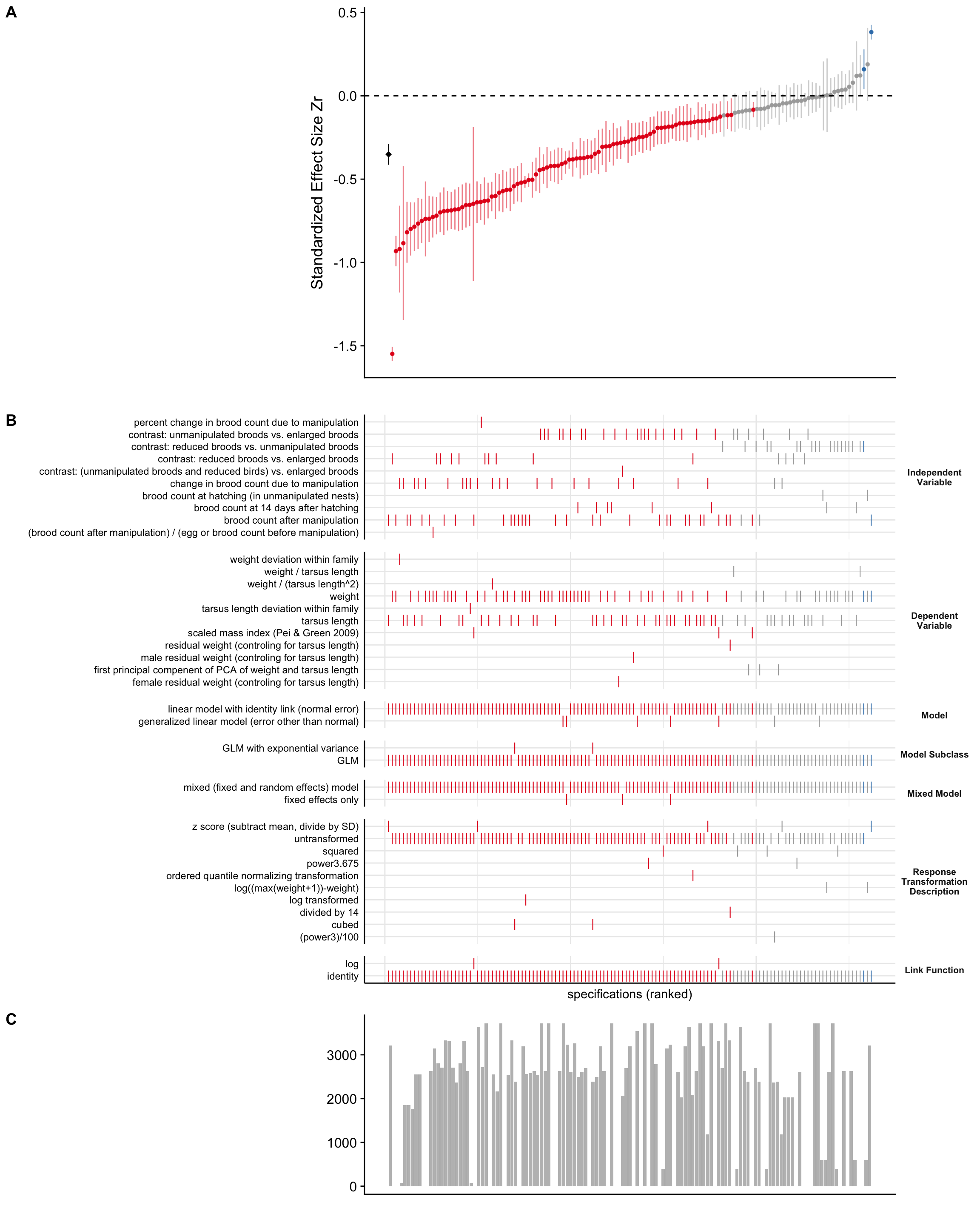
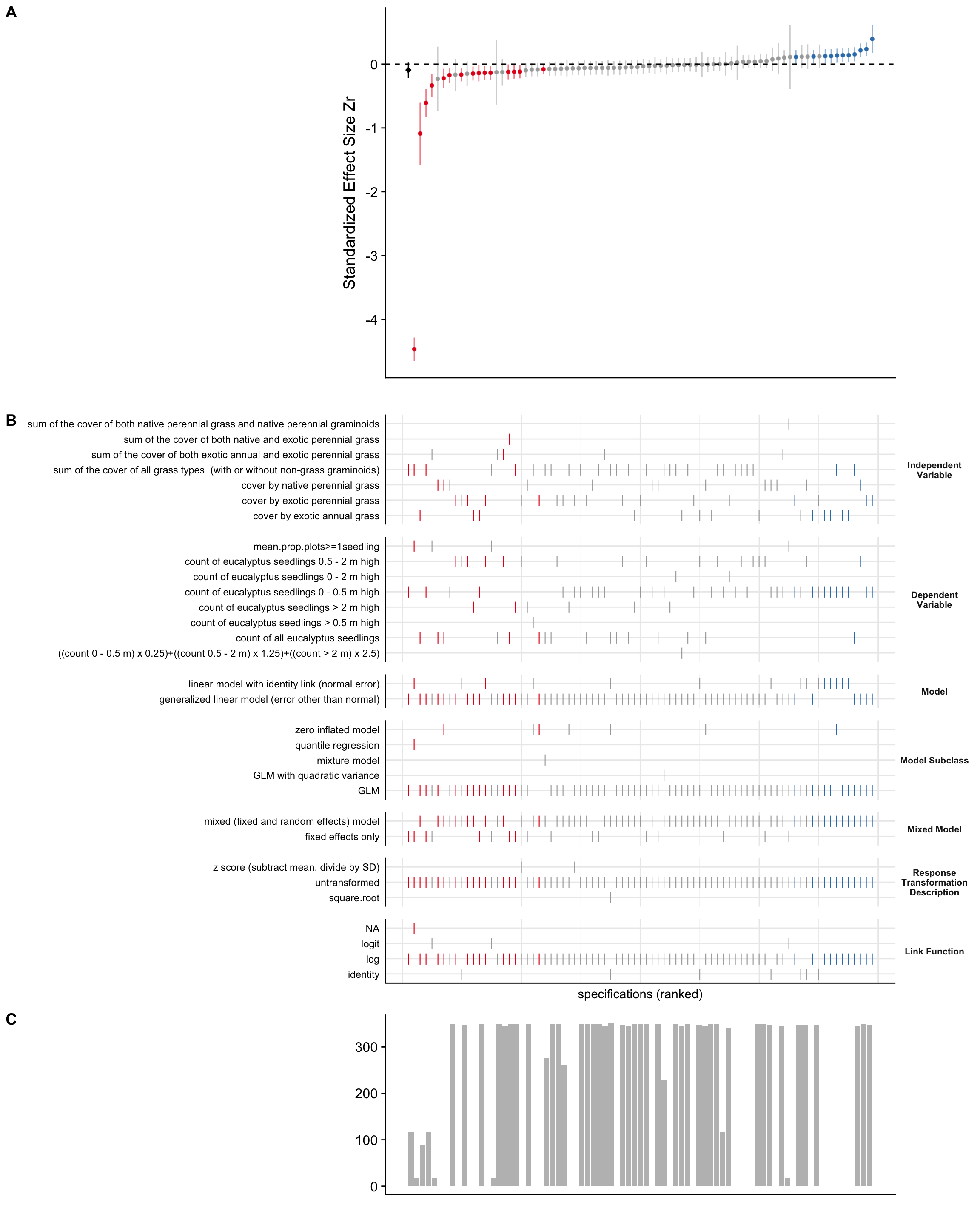
We used a specification curve (Simonsohn, Simmons, and Nelson 2015) to look for relationships between \(Z_r\) values and several modeling decisions, including the choice of independent and dependent variable, transformation of the dependent variable, and other features of the models that produced those \(Z_r\) values (Figure A.1, Figure A.2). Each effect can be matched to the model features that produced it by following a vertical line down the figure.
A.2.1 Blue tit
We observed few clear trends in the blue tit specification curve (Figure A.1). The clearest trend was for the independent variable ‘contrast: reduced broods vs. unmanipulated broods’ to produce weak or even positive relationships, but never strongly negative relationships. The biological interpretation of this pattern is that nestlings in reduced broods averaged similar growth to nestlings in unmanipulated broods, and sometimes the nestlings in reduced broods even grew less than the nestlings in unmanipulated broods. Therefore, it may be that competition limits nestling growth primarily when the number of nestlings exceeds the clutch size produced by the parents, and not in unmanipulated broods. The other relatively clear trend was that the strongest negative relationships were never based on the independent variable ‘contrast: unmanipulated broods vs. enlarged broods’. These observations demonstrate the potential value of specification curves.
Code
# knitr::read_chunk(here::here("index.qmd"), labels = "calc_MA_mod_coefs")#TODO why is here??coefs_MA_mod<-bind_rows(ManyEcoEvo_viz%>%filter(model_name=="MA_mod",exclusion_set=="complete",expertise_subset=="All"),ManyEcoEvo_viz%>%filter(model_name=="MA_mod",exclusion_set=="complete-rm_outliers",expertise_subset=="All")#TODO may need to recalculate)%>%hoist(tidy_mod_summary)%>%select(-starts_with("mod"), -ends_with("plot"), -estimate_type)%>%unnest(cols =c(tidy_mod_summary))
Code
analytical_choices_bt<-ManyEcoEvo_results$effects_analysis[[1]]%>%select(study_id, response_transformation_description, # Don't need constructed, as this is accounted for in yresponse_variable_name, test_variable, Bayesian, linear_model,model_subclass, sample_size, starts_with("num"),link_function_reported,mixed_model)%>%mutate(across(starts_with("num"), as.numeric), response_transformation_description =case_when(is.na(response_transformation_description)~"None",TRUE~response_transformation_description))%>%rename(y =response_variable_name, x =test_variable, model =linear_model)%>%select(study_id,x,y,model, model_subclass, response_transformation_description, link_function_reported, mixed_model, sample_size)%>%pivot_longer(-study_id, names_to ="variable_type", values_to ="variable_name",values_transform =as.character)%>%left_join(forest_plot_new_labels)%>%mutate(variable_name =case_when(is.na(user_friendly_name)~variable_name, TRUE~user_friendly_name))%>%select(-user_friendly_name)%>%pivot_wider(names_from =variable_type, values_from =variable_name)%>%mutate(sample_size =as.numeric(sample_size))MA_mean_bt<-ManyEcoEvo_viz$model[[1]]%>%broom::tidy(conf.int =TRUE)%>%rename(study_id =term)results_bt<-ManyEcoEvo_viz$model[[1]]%>%broom::tidy(conf.int =TRUE, include_studies =TRUE)%>%rename(study_id =term)%>%semi_join(analytical_choices_bt)%>%left_join(analytical_choices_bt)samp_size_hist_bt<-specr::plot_samplesizes(results_bt%>%rename(fit_nobs =sample_size))+cowplot::theme_half_open()+theme(axis.ticks.x =element_blank(), axis.text.x =element_blank())curve_bt<-specr::plot_curve(results_bt)+geom_hline(yintercept =0, linetype ="dashed", color ="black")+geom_pointrange(mapping =aes(x =0, y =estimate, ymin =conf.low, ymax =conf.high), data =MA_mean_bt, colour ="black", shape ="diamond")+labs(x ="", y ="Standardized Effect Size Zr")+cowplot::theme_half_open()+theme(axis.ticks.x =element_blank(), axis.text.x =element_blank())specs_bt<-specr::plot_choices(results_bt%>%rename("Independent\nVariable"=x,"Dependent\nVariable"=y, Model =model,"Model Subclass"=model_subclass,"Mixed Model"=mixed_model,"Response\nTransformation\nDescription"=response_transformation_description,"Link Function"=link_function_reported), choices =c("Independent\nVariable", "Dependent\nVariable", "Model", "Model Subclass", "Mixed Model", "Response\nTransformation\nDescription", "Link Function"))+labs(x ="specifications (ranked)")+theme(strip.text.x =element_blank(), strip.text.y =element_text(size =8, angle =360, face ="bold"), axis.ticks.x =element_blank(), axis.text.x =element_blank())cowplot::plot_grid(curve_bt, specs_bt, samp_size_hist_bt, ncol =1, align ="v", rel_heights =c(1.5, 2.2, 0.8), axis ="rbl",labels ="AUTO")
Figure A.1: A. Forest plot for blue tit analyses: standardized effect-sizes (circles) and their 95% confidence intervals are displayed for each analysis included in the meta-analysis model. The meta-analytic mean effect-size is denoted by a black diamond, with error bars also representing the 95% confidence interval. The dashed black line demarcates effect sizes of 0, whereby no effect of the test variable on the response variable is found. Blue points where Zr and its associated confidence intervals are greater than 0 indicate analyses that found a negative effect of sibling number on nestling growth. Gray coloured points have confidence intervals crossing 0, indicating no relationship between the test and response variable. Red points indicate the analysis found a positive relationship between sibling number and nestling growth. B. Analysis specification plot: for each analysis plotted in A, the corresponding combination of analysis decisions is plotted. Each decision and its alternative choices is grouped into its own facet, with the decision point described on the right of the panel, and the option shown on the left. Lines indicate the option chosen used in the corresponding point in plot A. C. Sample sizes of each analysis. Note that empty bars indicate analyst did not report sample size and sample size could not be derived by lead team.
A.2.2Eucalyptus
In the Eucalyptus specification curve, there are no strong trends (Figure A.2). It is, perhaps, the case that choosing the dependent variable ‘count of seedlings 0-0.5m high’ corresponds to more positive results and choosing ‘count of all Eucalytpus seedlings’ might find more negative results. Choosing the independent variable ‘sum of all grass types (with or without non-grass graminoids)’ might be associated with more results close to zero consistent with the absence of an effect.
Code
analytical_choices_euc<-ManyEcoEvo_results$effects_analysis[[2]]%>%select(study_id, response_transformation_description, # Don't need constructed, as this is accounted for in yresponse_variable_name, test_variable, Bayesian, linear_model,model_subclass, sample_size, starts_with("num"),transformation,mixed_model,link_function_reported)%>%mutate(across(starts_with("num"), as.numeric), response_transformation_description =case_when(is.na(response_transformation_description)~"None",TRUE~response_transformation_description), response_variable_name =case_when(response_variable_name=="average.proportion.of.plots.containing.at.least.one.euc.seedling.of.any.size"~"mean.prop.plots>=1seedling",TRUE~response_variable_name))%>%rename(y =response_variable_name, x =test_variable, model =linear_model)%>%select(study_id,x,y,model, model_subclass, response_transformation_description, link_function_reported, mixed_model, sample_size)%>%pivot_longer(-study_id, names_to ="variable_type", values_to ="variable_name",values_transform =as.character)%>%left_join(forest_plot_new_labels)%>%mutate(variable_name =case_when(is.na(user_friendly_name)~variable_name, TRUE~user_friendly_name))%>%select(-user_friendly_name)%>%pivot_wider(names_from =variable_type, values_from =variable_name, values_fn =list)%>%unnest(cols =everything())%>%#TODO remove unnest and values_fn = list when origin of duplicate entry for R_1LRqq2WHrQaENtM-1-1-1 is identifiedmutate(sample_size =as.numeric(sample_size))MA_mean_euc<-ManyEcoEvo_viz%>%filter(model_name=="MA_mod", publishable_subset=="All", dataset=="eucalyptus", exclusion_set=="complete")%>%pluck("model", 1)%>%broom::tidy(conf.int =TRUE)%>%rename(study_id =term)results_euc<-ManyEcoEvo_viz%>%filter(model_name=="MA_mod", publishable_subset=="All", dataset=="eucalyptus", exclusion_set=="complete")%>%pluck("model", 1)%>%broom::tidy(conf.int =TRUE, include_studies =TRUE)%>%rename(study_id =term)%>%semi_join(analytical_choices_euc)%>%left_join(analytical_choices_euc)samp_size_hist_euc<-specr::plot_samplesizes(results_euc%>%rename(fit_nobs =sample_size))+cowplot::theme_half_open()+theme(axis.ticks.x =element_blank(), axis.text.x =element_blank())curve_euc<-specr::plot_curve(results_euc)+geom_hline(yintercept =0, linetype ="dashed", color ="black")+geom_pointrange(mapping =aes(x =0, y =estimate, ymin =conf.low, ymax =conf.high), data =MA_mean_euc, colour ="black", shape ="diamond")+labs(x ="", y ="Standardized Effect Size Zr")+cowplot::theme_half_open()+theme(axis.ticks.x =element_blank(), axis.text.x =element_blank())specs_euc<-specr::plot_choices(results_euc%>%rename("Independent\nVariable"=x,"Dependent\nVariable"=y, Model =model,"Model Subclass"=model_subclass,"Mixed Model"=mixed_model,"Response\nTransformation\nDescription"=response_transformation_description,"Link Function"=link_function_reported), choices =c("Independent\nVariable", "Dependent\nVariable", "Model", "Model Subclass", "Mixed Model", "Response\nTransformation\nDescription", "Link Function"))+labs(x ="specifications (ranked)")+theme(strip.text.x =element_blank(), strip.text.y =element_text(size =8, angle =360, face ="bold"), axis.ticks.x =element_blank(), axis.text.x =element_blank())cowplot::plot_grid(curve_euc, specs_euc, samp_size_hist_euc, ncol =1, align ="v", rel_heights =c(1.5, 2.2, 0.8), axis ="rbl",labels ="AUTO")
Figure A.2: A. Forest plot for Eucalyptus analyses: standardized effect-sizes (circles) and their 95% confidence intervals are displayed for each analysis included in the meta-analysis model. The meta-analytic mean effect-size is denoted by a black diamond, with error bars also representing the 95% confidence interval. The dashed black line demarcates effect sizes of 0, whereby no effect of the test variable on the response variable is found. Blue points where \(Z_r\) and its associated confidence intervals are greater than 0 indicate analyses that found a positive relationship of grass cover on Eucalyptus seedling success. Gray coloured points have confidence intervals crossing 0, indicating no relationship between the test and response variable. Red points indicate the analysis found a negative relationship between grass cover and Eucalyptus seedling success. B. Analysis specification plot: for each analysis plotted in A, the corresponding combination of analysis decisions is plotted. Each decision and its alternative choices is grouped into its own facet, with the decision point described on the right of the panel, and the option shown on the left. Lines indicate the option chosen used in the corresponding point in plot A. C. Sample sizes of each analysis. Note that empty bars indicate analyst did not report sample size and sample size could not be derived by lead team.
Simonsohn, Uri, Joseph P. Simmons, and Leif D. Nelson. 2015. “Specification Curve: Descriptive and Inferential Statistics on All Reasonable Specifications.” Manuscript. SSRN Electronic Journal. https://doi.org/10.2139/ssrn.2694998 .