SM B: Effect Size Analysis

Code

library(withr)
library(here)
library(tidyverse)
library(performance)
library(broom.mixed)
library(gt)
library(gtExtras)
library(lme4)
library(MuMIn)
library(ManyEcoEvo)
library(ggrepel)
library(glue)
library(gluedown)
set.seed(1234)
source(here::here("utils.R"))

Code

ManyEcoEvo_results <- 
  ManyEcoEvo_results %>% 
  mutate(effects_analysis = 
           map(effects_analysis, 
               rename, 
               id_col = study_id)) #%>% 
  # mutate_at(c("data", 
  #             "diversity_data", 
  #             "diversity_indices", 
  #             "effects_analysis"),
  #           .funs = ~ map(.x, anonymise_teams,
  #                         TeamIdentifier_lookup))

B.1 Meta-analysis

B.1.1 Effect Sizes \(Z_r\)

B.1.1.1 Effect of categorical review rating

The figures below (Figure B.1, Figure B.2) hows the fixed effect of categorical review rating on deviation from the meta-analytic mean. There is very little difference in deviation for analyses in any of the review categories. It is worth noting that each analysis features multiple times in these figures corresponding to the multiple reviewers that provided ratings.

Code

orchard_publishability <- function(dat){
  rma_mod_rating <-  
    metafor::rma.mv(yi = Zr, 
                    V = VZr, 
                    data = dat, 
                    control = list(maxiter = 1000),mods = ~ PublishableAsIs,
                    sparse = TRUE,
                    random = list(~1|response_id, ~1|ReviewerId)) 
  
  orchaRd::orchard_plot(rma_mod_rating, 
                        mod = "PublishableAsIs", 
                        group = "id_col", 
                        xlab = "Standardised Correlation Coefficient (Zr)",
                        cb = TRUE,angle = 45) 
}

ManyEcoEvo_results$effects_analysis[[2]] %>% 
    filter(Zr > -4) %>% 
    unnest(review_data) %>% 
    select(Zr, VZr, id_col, PublishableAsIs, ReviewerId, response_id) %>% 
    mutate(PublishableAsIs = forcats::as_factor(PublishableAsIs) %>% 
               forcats::fct_relevel(c("deeply flawed and unpublishable", 
                                      "publishable with major revision", 
                                      "publishable with minor revision", 
                                      "publishable as is" ))) %>% 
    orchard_publishability() +
    theme(text = element_text(size = 20),axis.text.y = element_text(size = 20)) +
    scale_x_discrete(labels=c("Deeply Flawed\n & Unpublishable", "Publishable With\n Major Revision", "Publishable With\n Minor Revision", "Publishable\n As Is"))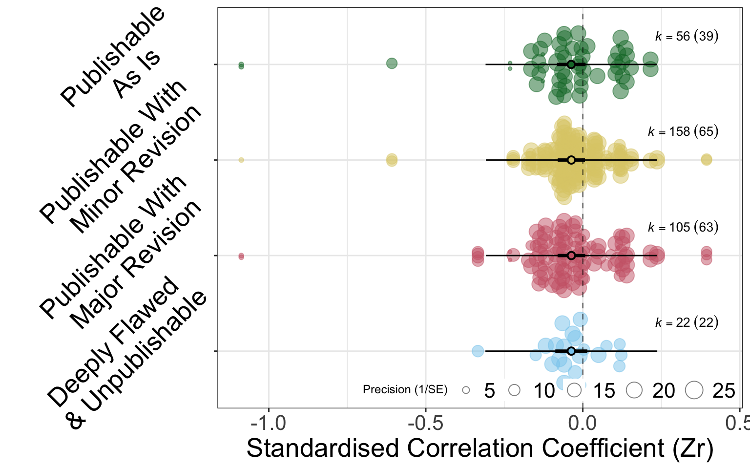

Code

ManyEcoEvo_results$effects_analysis[[1]] %>% 
#    filter(Zr > -4) %>% 
    unnest(review_data) %>% 
    select(Zr, VZr, id_col, PublishableAsIs, ReviewerId, response_id) %>% 
    mutate(PublishableAsIs = forcats::as_factor(PublishableAsIs) %>% 
               forcats::fct_relevel(c("deeply flawed and unpublishable", 
                                      "publishable with major revision", 
                                      "publishable with minor revision", 
                                      "publishable as is" ))) %>% 
    orchard_publishability() +
    theme(text = element_text(size = 20),axis.text.y = element_text(size = 20)) +
    scale_x_discrete(labels=c("Deeply Flawed\n & Unpublishable", "Publishable With\n Major Revision", "Publishable With\n Minor Revision", "Publishable\n As Is"))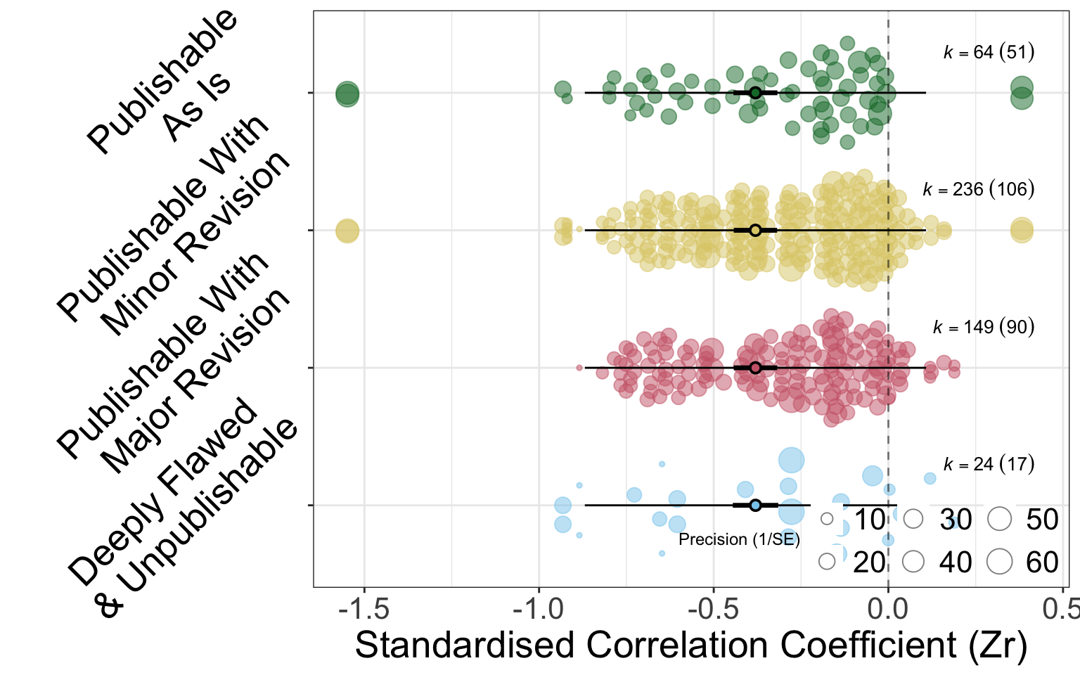

B.1.1.2 Post-hoc analysis: Exploring the effect of removing analyses with poor peer-review ratings on heterogeneity

The forest plots in Figure B.3 compare the distributions of \(Z_r\) effects from our full set of analyses with the distributions of \(Z_r\) effects from our post-hoc analyses, which removed either analyses that were reviewed at least once as being ‘unpublishable’, and analyses that were reviewed at least once as being ‘unpublishable’ or requiring ‘major revisions’. Removing these analyses from the blue tit data had little impact on the overall distribution of the results. When ‘unpublishable’ analyses of the Eucalyptus dataset were removed, the extreme outlier ‘Brooklyn-2-2-1’ was also removed, resulting in a substantial difference to the amount of observed deviation from the meta-analytic mean.

Code

# TeamIdentifier_lookup <- read_csv(here::here("data-raw/metadata_and_key_data/TeamIdentifierAnonymised.csv"))

plot_forest <- function(data, intercept = TRUE, MA_mean = TRUE){
  if (MA_mean == FALSE){
    data <- filter(data, Parameter != "overall")
  }
  
  p <- ggplot(data, aes(y = estimate, 
                        x =  term, 
                        ymin = conf.low, 
                        ymax = conf.high,
                        shape = point_shape,
                        colour = parameter_type)) +
    geom_pointrange(fatten = 2) +
    ggforestplot::theme_forest() +
    theme(axis.line = element_line(linewidth = 0.10, 
                                   colour = "black"),
          axis.line.y = element_blank(),
          text = element_text(family = "Helvetica")#,
          # axis.text.y = element_blank()
    ) +
    guides(shape = "none", colour = "none") +
    coord_flip() +
    ylab(bquote(Standardised~Effect~Size~Z[r])) +
    xlab(element_blank()) +
    # scale_y_continuous(breaks = c(-4,-3,-2,-1,0,1),
    # minor_breaks = seq(from = -4.5, to = 1.5, by = 0.5)) +
    NatParksPalettes::scale_color_natparks_d("Glacier")
  
  if(intercept == TRUE){
    p <- p + geom_hline(yintercept = 0)
  }
  if(MA_mean == TRUE){
    p <- p + geom_hline(aes(yintercept = meta_analytic_mean), 
                        data = data,
                        colour = "#01353D", 
                        linetype = "dashed")
  }
  
  return(p)
}

publishable_subsets_forest_data <- 
  ManyEcoEvo_viz %>% 
  filter(model_name == "MA_mod",
         exclusion_set == "complete",
         expertise_subset == "All") %>% 
  select(ends_with("set"), model, -expertise_subset) %>%  
  mutate(plot_data = 
           map(model, 
               .f = 
                 ~broom::tidy(.x, 
                              conf.int = TRUE, 
                              include_studies = TRUE) %>% 
                 mutate(Parameter = 
                          forcats::fct_reorder(term, estimate))),
         meta_analytic_mean = 
           map_dbl(plot_data, 
                   ~ filter(.x, 
                            Parameter == "overall") %>% 
                     pull(estimate))) %>% 
  select(dataset, 
         publishable_subset, 
         plot_data, 
         meta_analytic_mean) %>% 
  unnest(cols = c("plot_data")) %>% 
  mutate(parameter_type = 
           case_when(
             str_detect(Parameter, "overall") ~ "mean",
             TRUE ~ "study"))  %>% 
  group_by(dataset, publishable_subset) %>%
  dplyr::mutate(point_shape = 
                  ifelse(stringr::str_detect(term, "overall"), 
                         "diamond", 
                         "circle")) 

# publishable_subsets_forest_data <- 
#   publishable_subsets_forest_data %>% 
#    rename(id_col = term) %>% 
#   group_by(type) %>%  
#   group_split() %>% 
#   set_names(., publishable_subsets_forest_data$type %>%  unique) %>% 
#   # map_if(.x = ., names(.) == "study",
#   #        .f = ~ anonymise_teams(.x, TeamIdentifier_lookup)) %>% 
#   bind_rows() %>% 
#   rename(term = id_col)

library(tidytext)

tidy_overall_labeller <- . %>% 
  str_split("_") %>% 
  flatten_chr() %>% 
  pluck(1)

tidy_forest_labels <- Vectorize(tidy_overall_labeller)

publishable_subsets_forest_data %>% 
  group_by(dataset, publishable_subset) %>% 
  mutate(term = case_when(term == "overall" ~ 
                            paste(term, 
                                   dataset, 
                                   publishable_subset,
                                  sep = "_"), 
                          TRUE ~ term),
         dataset = case_when(dataset == "blue tit" ~ "Blue tit",
                              dataset == "eucalyptus" ~ "Eucalyptus",
                              TRUE ~ NA)) %>% 
  arrange(across(.cols = c(type, estimate)),
          .by_group = TRUE) %>% 
  rowid_to_column() %>% 
  mutate(term = reorder(term, rowid),
         publishable_subset = 
           case_when(publishable_subset == "All" ~ 
                       "All analyses",
                     publishable_subset == "data_flawed" ~ 
                       "'Unpublishable'\nremoved",
                     publishable_subset == "data_flawed_major" ~ 
                       "'Unpublishable' &\n'Major Revisions'\nremoved",
                     TRUE ~ "")) %>%  
  plot_forest() +
  scale_x_reordered(labels =  tidy_forest_labels) +
  ggh4x::facet_nested(dataset ~ publishable_subset,
                      independent = "y", 
                      scales = "free")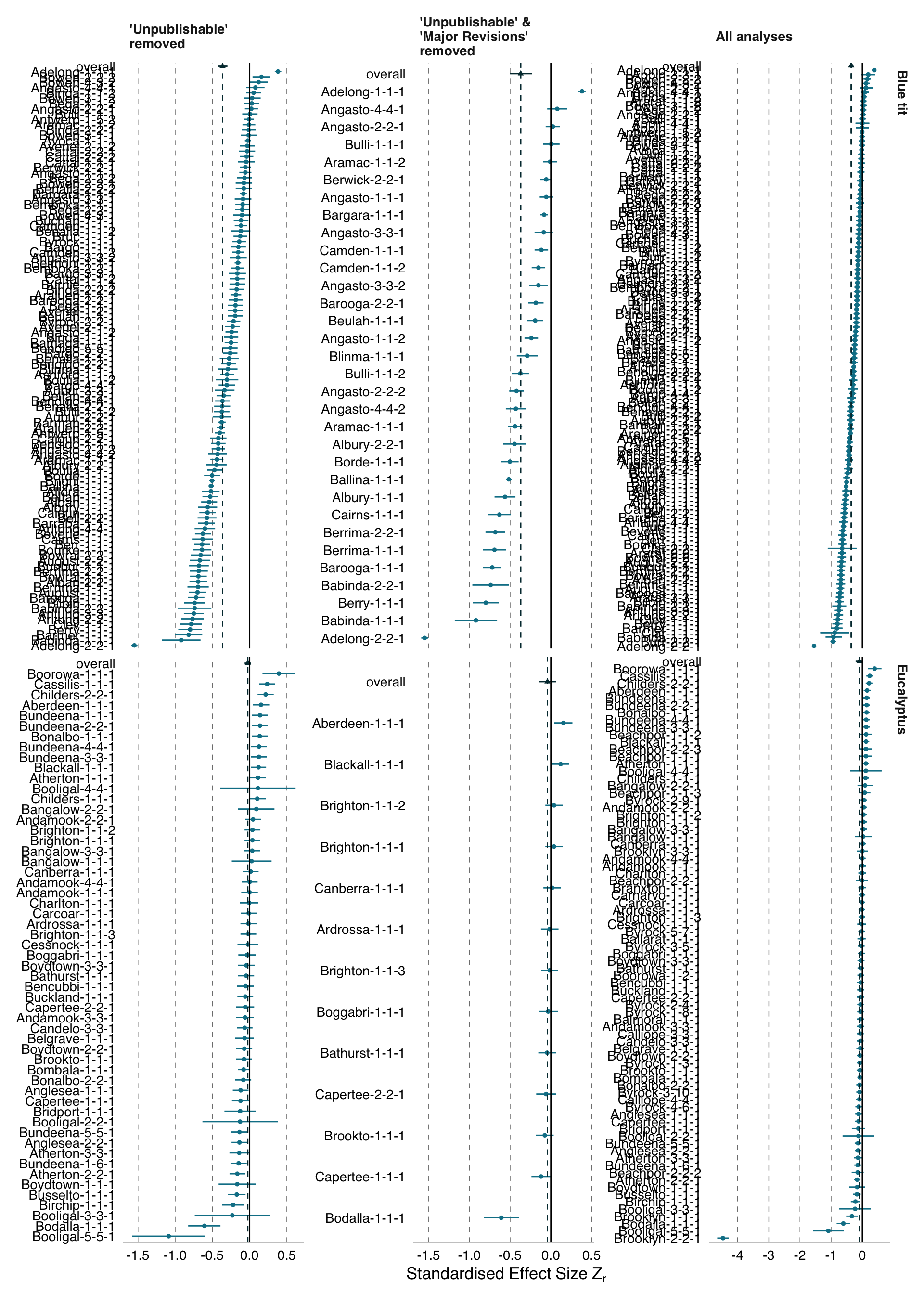

Figure B.3: Forest plots of meta-analytic estimated standardized effect sizes (\(Z_r\), blue circles) and their 95% confidence intervals for each effect size included in the meta-analysis model. The meta-analytic mean effect size is denoted by a black triangle and a dashed vertical line, with error bars also representing the 95% confidence interval. The solid black vertical line demarcates effect size of 0, indicating no relationship between the test variable and the response variable. The left side of each panel shows the analysis team names (anonymous arbitrary names assigned by us), each followed by three numbers. The first number is the submission ID (some analyst teams submitted results to us on >1 submission form), the second number is the analysis ID (some analyst teams included results of >1 analysis in a given submission), and the third number is the effect ID (some analysts submitted values for >1 effect per analysis). Thus, each row in each forest plot is uniquely identified, but it is possible to determine which effects come from which analyses and which analysis teams. The plots in the top row depict effects from analyses of blue tit data, and the bottom row plots depict effects from analyses of Eucalyptus data. The right-most plots depict all usable effect sizes. The plots on the left exclude effects from analysis sets that received at least one rating of “unpublishable” from peer reviewers, and the plots in the middle exclude effects from analysis sets that received at least one rating of either “unpublishable” or “major revision” from peer reviewers.

B.1.1.3 Post-hoc analysis: Exploring the effect of excluding estimates in which we had reduced confidence

For each dataset (blue tit, Eucalyptus), we created a second, more conservative version, that excluded effects based on estimates of \(\mathit{df}\) that we considered less reliable (Table B.1). We compared the outcomes of analyses of the primary dataset (constituted according to our registered plan) with the outcomes of analyses of the more conservative version of the dataset. We also compared results from analyses of both of these versions of the dataset to versions with our post-hoc removal of outliers described in the main text. Our more conservative exclusions (based on unreliable estimates of \(\mathit{df}\) ) had minimal impact on the meta-analytic mean for both blue tit and Eucalyptus analyses, regardless of whether outliers were excluded (Table B.1).

Code

ManyEcoEvo_viz %>% 
    dplyr::filter(estimate_type == "Zr", 
                  model_name == "MA_mod", 
                  collinearity_subset != "collinearity_removed",
                  publishable_subset == "All", 
                  expertise_subset == "All") %>% 
    select(dataset, exclusion_set, tidy_mod_summary) %>% 
    unnest(tidy_mod_summary) %>% 
    filter(type == "summary") %>% 
  select(-term, -type) %>% 
  mutate(exclusion_set = 
           case_when(exclusion_set == "complete" ~ 
                       "Primary dataset",
                     exclusion_set == "complete-rm_outliers" ~ 
                       "Primary dataset, outliers removed",
                     exclusion_set == "partial" ~ 
                       "Conservative exclusions",
                     TRUE ~ "Conservative exclusions, outliers removed")) %>% 
group_by(exclusion_set) %>% 
  gt::gt() %>% 
  gt::opt_stylize(style = 6, color = "gray") %>% 
  gt::fmt(columns = "p.value",
          fns = function(x) gtsummary::style_pvalue(x, prepend_p = FALSE)) %>% 
  gt::fmt_number(columns = c(-p.value, -dataset)) %>% 
  gt::cols_label(estimate = gt::md("$$\\hat\\mu$$"), 
                 std.error = gt::md("$$\text{SE}[\\hat\\mu]$$"),
                 conf.low = gt::md("95\\%CI")) %>% 
  gt::cols_merge(columns = starts_with("conf"), 
                 pattern = "[{1},{2}]") %>% 
  gt::cols_move(columns = conf.low, after = std.error) %>% 
   gt::tab_style(
    style = list(gt::cell_text(transform = "capitalize"), 
                 gt::cell_text(style = "italic")),
    locations = gt::cells_body(columns = "dataset", rows = dataset == "eucalyptus")
  )

Table B.1: Estimated meta-analytic mean, standard error, and 95% confidence intervals, from analyses of the primary data set, the more conservative version of the dataset which excluded effects based on less reliable estimates of \(\mathit{df}\), and both of these datasets with outliers removed.

dataset	\[\hat\mu\]	\[ ext{SE}[\hat\mu]\]	95%CI	statistic	p.value
Primary dataset
blue tit	−0.35	0.03	[−0.41,−0.29]	−11.02	<0.001
eucalyptus	−0.09	0.06	[−0.22,0.03]	−1.47	0.14
Conservative exclusions
blue tit	−0.36	0.03	[−0.42,−0.29]	−10.77	<0.001
eucalyptus	−0.11	0.07	[−0.24,0.03]	−1.55	0.12
Primary dataset, outliers removed
blue tit	−0.36	0.03	[−0.42,−0.30]	−11.48	<0.001
eucalyptus	−0.03	0.01	[−0.06,0.00]	−2.23	0.026
Conservative exclusions, outliers removed
blue tit	−0.36	0.03	[−0.43,−0.30]	−11.38	<0.001
eucalyptus	−0.04	0.02	[−0.07,−0.01]	−2.52	0.012

Code

plot_forest <- function(data, intercept = TRUE, MA_mean = TRUE ){
  if (MA_mean == FALSE) {
    data <- filter(data, term != "Overall")
  }
  
    p <- ggplot(data, aes(y = term, 
                        x =  estimate, 
                        ymin = conf.low, 
                        ymax = conf.high,
                        # shape = point_shape,
                        colour = parameter_type)) +
    geom_pointrange() +
    ggforestplot::theme_forest() +
    theme(axis.line = element_line(size = 0.10, colour = "black"),
          axis.line.y = element_blank(),
          text = element_text(family = "Helvetica"),
          axis.text.y = element_blank()) +
    guides(shape = "none", colour = "none") +
    coord_flip() +
    labs(y = "Standardised Effect Size, Zr",
         x = element_blank()) +
    scale_x_continuous(breaks = c(-4,-3,-2,-1,0,1),
                       minor_breaks = seq(from = -4.5, to = 1.5, by = 0.5)) +
    NatParksPalettes::scale_color_natparks_d("Glacier")
    
    if (intercept == TRUE) {
      p <- p + geom_hline(yintercept = 0)
    }
    if (MA_mean == TRUE) {
      p <- p + geom_hline(aes(yintercept = meta_analytic_mean), 
                          data = data,
                          colour = "#01353D", 
                          linetype = "dashed")
    }
    
  return(p)
}

Code

complete_euc_data <- 
  ManyEcoEvo_viz %>% 
  filter(exclusion_set == "complete", 
         estimate_type == "Zr", 
         model_name == "MA_mod",
         dataset == "eucalyptus",
         publishable_subset == "All",
         expertise_subset == "All") %>% 
  select(tidy_mod_summary) %>% 
  mutate(plot_data = map(tidy_mod_summary, 
                         .f = ~ dplyr::mutate(.x, 
                                            point_shape = 
                                              ifelse(stringr::str_detect(term, "overall"), 
                                                     "diamond", 
                                                     "circle"),
                                            Parameter = 
                                              forcats::fct_reorder(term, 
                                                                   estimate) %>% 
                                              forcats::fct_reorder(., 
                                                                   point_shape,
                                                                   .desc = TRUE))
  ),
  meta_analytic_mean = map_dbl(plot_data, 
                               ~ filter(.x, Parameter == "overall") %>% 
                                 pull(estimate))) %>% 
  select(plot_data, meta_analytic_mean) %>% 
  unnest(cols = c("plot_data")) %>% 
  mutate(parameter_type = case_when(str_detect(Parameter, "overall") ~ "mean",
                                    TRUE ~ "study"))

  # ManyEcoEvo_viz %>% 
  # filter(exclusion_set == "complete", 
  #        estimate_type == "Zr", 
  #        model_name == "MA_mod",
  #        dataset == "eucalyptus",
  #        publishable_subset == "All",
  #        expertise_subset == "All") %>% 
  # )

min_outlier_euc <- complete_euc_data %>% 
  filter(type == "study") %>% 
  slice_min(estimate, n = 3) %>% 
  pull(term)

sample_size_euc_Zr <- ManyEcoEvo_results %>% 
    filter(exclusion_set == "complete", dataset == "eucalyptus") %>% 
    pluck("data", 1) %>% 
    select(id_col, sample_size) %>% 
    rename(term = id_col) %>% 
    mutate(sample_size = as.numeric(sample_size))

mean_n_euc_Zr <- sample_size_euc_Zr %>% 
  drop_na(sample_size) %>% 
  pull(sample_size) %>% 
  mean() %>% 
  round(2)

N_outliers_Zr_euc <- sample_size_euc_Zr %>% 
  filter(term %in% min_outlier_euc) %>% 
   arrange(desc(sample_size))

B.1.1.4 Post-hoc analysis: Exploring the effect of including only analyses conducted by analysis teams with at least one member self-rated as “highly proficient” or “expert” in conducting statitistical analyses in their research area

The anonymous Team Identifiers in the reduced subset of “expert” or “highly proficient” analysts are exported internally in the ManyEcoEvo package as ManyEcoEvo:::expert_subset. Analyses from the following teams are retained in the reduced subset: Bell, Berr, Brim, Bruc, Burr, Byng, Cape, Clar, Clev, Alban, Alpha, Bargo, Berry, Bowen, Bulli, Aldgat, Alding, Anakie, Aramac, August, Bamaga, Barham, Barmah, Batlow, Beltan, Bethan, Beulah, Bindoo, Boonah, Bowral, Bright, Buchan, Burnie, Cairns, Casino, Cattai, Adelong, Angasto, Antwerp, Arltung, Ashford, Babinda, Bargara, Barooga, Barraba, Belmont, Bemboka, Benalla, Bendigo, Berrima, Berwick, Beverle, Bicheno, Biloela, Birchip, Bombala, Bonalbo, Brookto, Bruthen, Buderim, Candelo, Capella, Carcoar, Carnama, Chewton, Anglesea, Ardrossa, Armidale, Atherton, Balaklav, Ballarat, Barellan, Belgrave, Berrigan, Binalong, Binnaway, Blackall, Boggabri, Bridport, Brooklyn, Buckland, Bundeena, Bungonia, Busselto, Calliope, Cardwell, Cassilis, Cessnock, Charlton.

Code

plot_forest <- function(data, intercept = TRUE, MA_mean = TRUE){
  if (MA_mean == FALSE){
    data <- filter(data, Parameter != "overall")
  }
  
  p <- ggplot(data, aes(y = estimate, 
                        x =  term, 
                        ymin = conf.low, 
                        ymax = conf.high,
                        shape = parameter_type,
                        colour = parameter_type)) +
    geom_pointrange(fatten = 2) +
    ggforestplot::theme_forest() +
    theme(axis.line = element_line(linewidth = 0.10, colour = "black"),
          axis.line.y = element_blank(),
          text = element_text(family = "Helvetica")#,
          # axis.text.y = element_blank()
    ) +
    guides(shape = guide_legend(title = NULL), 
           colour = guide_legend(title = NULL)) +
    coord_flip() +
    ylab(bquote(Standardised~Effect~Size~Z[r])) +
    xlab(element_blank()) +
    # scale_y_continuous(breaks = c(-4,-3,-2,-1,0,1),
    # minor_breaks = seq(from = -4.5, to = 1.5, by = 0.5)) +
    NatParksPalettes::scale_color_natparks_d("Glacier")
  
  if(intercept == TRUE){
    p <- p + geom_hline(yintercept = 0)
  }
  if(MA_mean == TRUE){
    p <- p + geom_hline(aes(yintercept = meta_analytic_mean), 
                        data = data,
                        colour = "#01353D", 
                        linetype = "dashed")
  }
  
  return(p)
}

filter_experts <- 
  rlang::exprs(
    exclusion_set == "complete", 
    estimate_type == "Zr", 
    model_name == "MA_mod",
    publishable_subset == "All", 
    expertise_subset == "expert")

bt_experts_only <- 
  ManyEcoEvo_viz %>% 
  filter(!!!filter_experts, 
         dataset == "blue tit") %>% 
  select(tidy_mod_summary) %>% 
  mutate(plot_data = map(tidy_mod_summary, 
                         .f = ~ dplyr::mutate(.x, 
                                            point_shape = 
                                              ifelse(stringr::str_detect(term, "overall"), 
                                                     "diamond", 
                                                     "circle"),
                                            Parameter = 
                                              forcats::fct_reorder(term, 
                                                                   estimate) %>% 
                                              forcats::fct_reorder(., 
                                                                   point_shape,
                                                                   .desc = TRUE))
  ),
  meta_analytic_mean = map_dbl(plot_data, 
                               ~ filter(.x, Parameter == "overall") %>% 
                                 pull(estimate))) %>% 
  select(plot_data, meta_analytic_mean) %>% 
  unnest(cols = c("plot_data")) %>% 
  mutate(parameter_type = case_when(str_detect(Parameter, "overall") ~ "mean",
                                    TRUE ~ "study")) 

# bt_experts_only <- 
#   bt_experts_only %>% 
#   rename(id_col = term) %>% 
#   group_by(type) %>%  
#   group_split() %>% 
#   set_names(., bt_experts_only$type %>%  unique) %>% 
#   # map_if(.x = ., names(.) == "study",
#          # .f = ~ anonymise_teams(.x, TeamIdentifier_lookup)) %>% 
#   bind_rows() %>% 
#   rename(term = id_col)

bt_forest_experts <- bt_experts_only %>% 
  arrange(desc(type)) %>% 
  mutate(type = forcats::as_factor(type)) %>% 
  group_by(type) %>% 
  arrange(desc(estimate),.by_group = TRUE) %>% 
  mutate(term = forcats::as_factor(term),
         point_shape = case_when(str_detect(type, "summary") ~ "mean",
                                 TRUE ~ "study")) %>% 
  plot_forest(intercept = TRUE, MA_mean = TRUE) +
  theme(axis.text.x = element_text(size = 15), 
        axis.title.x = element_text(size = 15),
        axis.text.y = element_blank()
  ) +
  scale_y_continuous(limits = c(-1.6, 0.65)) 

euc_experts_only <- 
  ManyEcoEvo_viz %>% 
  filter(!!!filter_experts, 
         dataset == "eucalyptus") %>% 
  select(model) %>% 
  mutate(plot_data = map(model, 
                         .f = ~ broom::tidy(.x, 
                                            conf.int = TRUE, 
                                            include_studies = TRUE) %>% 
                           dplyr::mutate(point_shape = 
                                           ifelse(stringr::str_detect(term, "overall"), 
                                                  "diamond", 
                                                  "circle"),
                                         Parameter = 
                                           forcats::fct_reorder(term, 
                                                                estimate) %>% 
                                           forcats::fct_reorder(., 
                                                                point_shape,
                                                                .desc = TRUE))
  ),
  meta_analytic_mean = map_dbl(plot_data, 
                               ~ filter(.x, Parameter == "overall") %>% 
                                 pull(estimate))) %>% 
  select(plot_data, meta_analytic_mean) %>% 
  unnest(cols = c("plot_data")) %>% 
  mutate(parameter_type = case_when(str_detect(Parameter, "overall") ~ "mean",
                                    TRUE ~ "study"))

# euc_experts_only <- 
#   euc_experts_only %>% 
#   rename(id_col = term) %>% 
#   group_by(type) %>%  
#   group_split() %>% 
#   set_names(., euc_experts_only$type %>%  unique) %>% 
#   # map_if(.x = ., names(.) == "study",
#          # .f = ~ anonymise_teams(.x, TeamIdentifier_lookup)) %>% 
#   bind_rows() %>% 
#   rename(term = id_col)

euc_forest_experts <- euc_experts_only %>% 
  arrange(desc(type)) %>% 
  mutate(type = forcats::as_factor(type)) %>% 
  group_by(type) %>% 
  arrange(desc(estimate),.by_group = TRUE) %>% 
  mutate(term = forcats::as_factor(term),
         point_shape = case_when(str_detect(type, "summary") ~ "mean",
                                 TRUE ~ "study")) %>% 
  plot_forest(intercept = TRUE, MA_mean = TRUE) +
  theme(axis.text.x = element_text(size = 15), 
        axis.title.x = element_text(size = 15),
        axis.text.y = element_blank()
  ) +
  scale_y_continuous(limits = c(-5, 1), 
                     breaks = c(-5, -4, -3, -2, -1, 0, 1) )

# ---- Extract Viz ----

bt_forest_experts

euc_forest_experts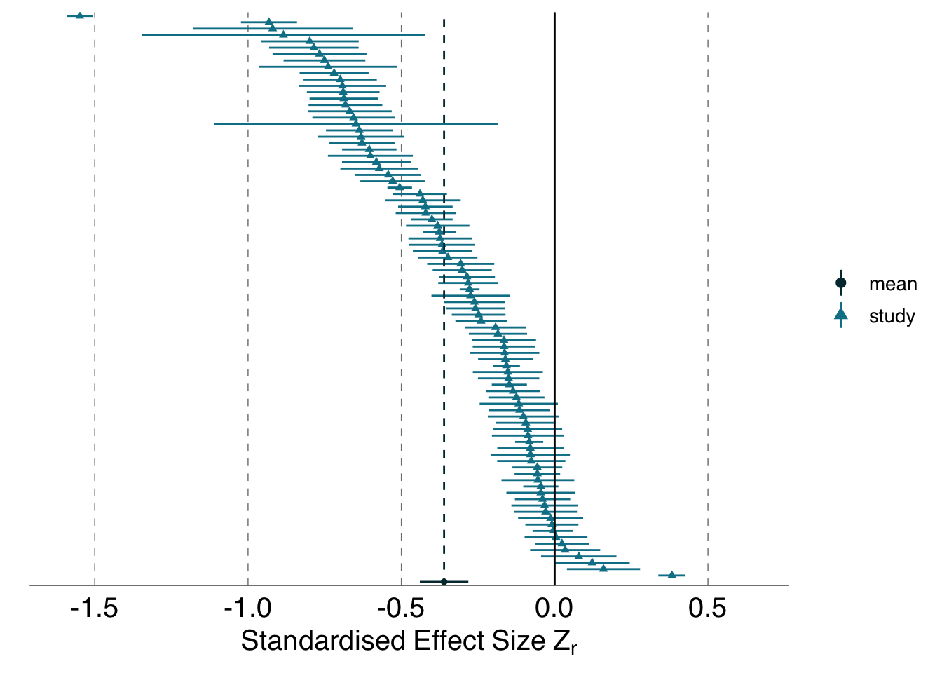

B.1.1.5 Post-hoc analysis: Exploring the effect of excluding analyses of the blue tit dataset containing highly collinear predictor variables

For the blue tit dataset, we created a subset of analyses that excluded effects based on analyses containing highly correlated predictor variables. Excluded analyses are exported internally in the ManyEcoEvo package as ManyEcoEvo::collinearity_subset. Analyses with the following identifiers are excluded in the reduced subset: Armadal-1-1-1, Babinda-1-1-1, Babinda-2-2-1, Barham-1-1-1, Barham-2-2-1, Bega-1-1-1, Bega-1-1-2, Bega-2-2-1, Bega-2-2-2, Borde-1-1-1, Bruc-1-1-1, Caigun-1-1-1, Caigun-2-2-1, Adelong-1-1-1, Adelong-2-2-1.

Code

filter_collinear <- rlang::exprs(exclusion_set == "complete", 
                              publishable_subset == "All", 
                              expertise_subset == "All", 
                              collinearity_subset == "collinearity_removed",
                              model_name == "MA_mod",
                              dataset == "blue tit")

# summary_output_params <- rlang::exprs(tidy_mod_summary, MA_fit_stats, mod_fit_stats)

ManyEcoEvo_viz %>% 
  filter(!!!filter_collinear) %>% 
  mutate(plot_data = map(tidy_mod_summary, 
                         .f = ~ dplyr::mutate(.x, 
                                            point_shape = 
                                              ifelse(stringr::str_detect(term, "overall"), 
                                                     "diamond", 
                                                     "circle"),
                                            Parameter = 
                                              forcats::fct_reorder(term, 
                                                                   estimate) %>% 
                                              forcats::fct_reorder(., 
                                                                   point_shape,
                                                                   .desc = TRUE))
  ),
  meta_analytic_mean = map_dbl(plot_data, 
                               ~ filter(.x, Parameter == "overall") %>% 
                                 pull(estimate))) %>% 
  select(plot_data, meta_analytic_mean) %>% 
  unnest(cols = c("plot_data")) %>% 
  mutate(parameter_type = case_when(str_detect(Parameter, "overall") ~ "mean",
                                    TRUE ~ "study")) %>% 
  arrange(desc(type)) %>% 
  mutate(type = forcats::as_factor(type)) %>% 
  group_by(type) %>% 
  arrange(desc(estimate),.by_group = TRUE) %>% 
  mutate(term = forcats::as_factor(term),
         point_shape = case_when(str_detect(type, "summary") ~ "mean",
                                 TRUE ~ "study")) %>% 
  plot_forest(intercept = TRUE, MA_mean = TRUE) +
  theme(axis.text.x = element_text(size = 15), 
        axis.title.x = element_text(size = 15),
        axis.text.y = element_blank()
  ) +
    scale_y_continuous(limits = c(-1.5, 0.5), 
                     breaks = c(-1.5, -1, -0.5, 0, 0.5) )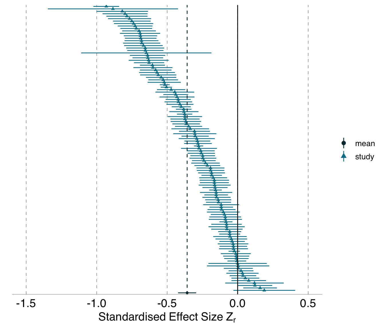

Figure B.5: Forest plot of meta-analytic estimated effect-sizes \(Z_{r}\), standard error and 95% confidence intervals of blue tit analyses with highly collinear analyses removed. The meta-analytic mean for the reduced subset is denoted by the black triangle, and a dashed vertical line, with error bars representing the 95% confidence interval. The solid black vertical line demarcates effect size of 0.

B.1.2 Out of sample predictions \(y_i\)

B.1.2.1 Excluded analyses with constructed variables

Code

by <- join_by(response_variable_name) # don't join on id_col: inc. other excl.

# Analyst Constructed Variables
all_constructed_vars <- 
  ManyEcoEvo %>% 
    pull(data, dataset) %>% 
    list_rbind(names_to = "dataset") %>% 
    filter(str_detect(response_variable_type, "constructed")) %>% 
    distinct(dataset,response_variable_name) %>% 
    drop_na() %>% 
    arrange()

# Constructed Variables Included in the ManyAnalysts meta-analysis
# (i.e. we have included them in the parameter tables)
ManyEcoEvo_yi_constructed_vars <-
 ManyEcoEvo:::analysis_data_param_tables %>% 
  distinct(variable, dataset) %>% 
  rename(response_variable_name = variable) %>% 
  semi_join(all_constructed_vars, by) %>% 
  filter(!str_detect(response_variable_name, 
                     "average.proportion.of")) # was excluded

yi_constructed <-
  ManyEcoEvo_yi_results %>% 
    pull(data, dataset) %>% 
    list_rbind(names_to = "dataset") %>% 
    filter(str_detect(response_variable_type, "constructed")) %>% 
    distinct(dataset, id_col, TeamIdentifier, response_variable_name) %>% 
    drop_na() 

excluded_yi_constructed <- 
  ManyEcoEvo %>% 
  pull(data, dataset) %>% 
  list_rbind(names_to = "dataset") %>% 
  filter(str_detect(response_variable_type, "constructed"),
         str_detect(exclusions_all, "retain")) %>% 
  distinct(dataset, id_col, TeamIdentifier, response_variable_name) %>% 
  drop_na() %>% 
  anti_join(yi_constructed, by) #rm response vars in yi_constructed

n_dropped_analyses <- 
  excluded_yi_constructed %>% 
  n_distinct("id_col")

n_teams_w_dropped_analyses <- 
  excluded_yi_constructed %>% 
  group_by(TeamIdentifier) %>%  
  count() %>% 
  n_distinct("TeamIdentifier")

We standardized the \(y_i\) estimates and their standard errors for the blue tit analyses using the population mean and standard deviations of the corresponding dependent variable for that analysis, as shown in Equation B.1, using the function ManyEcoEvo::Z_VZ_preds(). Note that this is NOT the same process as standardizing the effect sizes \(Z_r\). We used the mean and standard deviation of the relevant raw datasets as our ‘population’ parameters.

\[ Z_j = \frac{\mu_i-\bar{x}_j}{\text{SD}_j} \\ \\ {\text{VAR}}_{Z_j} = \frac{{\text{SE}}_{\mu_i}}{{\text{SD}_j}} \\ \tag{B.1}\]

Where \(\mu\) is the population parameter taken from our original dataset for variable \(i\), and \(\bar{x}_j\) and \(\text{SD}_j\) are the out of sample point estimate values supplied for analysis \(j\). \(\text{SE}_{{\mu}_{i}}\) is the standard error of the population mean for variable \(i\), while \({\text{VAR}}_{{Z}_{j}}\) and \({Z}_{j}\) are the standardized variance and mean estimate for analysis \(j\). Note that for the response variables that were scaled-and-centered, or else mean-centred before model fitting, we do not need to standardise because these are already on the Z-scale. In doing so we make the assumption that analysts’ data subsetting will have little effect on the outcomes. For some analyses of the blue tit dataset, analysts constructed their own unique response variables, which meant we needed to reconstruct these variables in order to calculate the population parameters. Unfortunately we were not able to re-construct all variables used by the analysts, as we were unable to reproduce the data required for their re-construction, e.g. we were unable to reproduce principal component analyses or fitted models for extracting residuals Table B.2. A total of 15 were excluded from out-of-sample meta-analysis, from 10 teams, including the following analysis identifiers: Bruc-1-1-1, Clar-2-2-1, Clar-1-1-1, Batlow-1-1-1, Batlow-1-1-2, Bindoo-1-1-1, Bourke-1-1-1, Buchan-1-1-1, Arltung-4-4-1, Bargara-1-1-1, Bendigo-5-5-1, Booligal-3-3-1, Booligal-2-2-1, Booligal-4-4-1 and Booligal-5-5-1.

Code

all_constructed_vars %>% 
  semi_join(ManyEcoEvo_yi_constructed_vars, by) %>% 
  mutate(included_in_yi = TRUE) %>% 
  bind_rows(
    {
      all_constructed_vars %>% 
        anti_join(ManyEcoEvo_yi_constructed_vars, by) %>% 
        mutate(included_in_yi = FALSE)
    }
  ) %>% 
  dplyr::mutate(included_in_yi = 
                  case_match(included_in_yi, 
                                            TRUE ~ "check", 
                                            FALSE ~ "xmark" ),
                response_variable_name = 
                  gluedown::md_code(response_variable_name)) %>% 
  group_by(dataset) %>% 
  gt::gt() %>% 
  gt::cols_label(response_variable_name = "Constructed Variable",
                 included_in_yi = gt::md("Variable reconstructed for meta-analysis?")) %>%
  gt::fmt_icon(included_in_yi) %>% 
  gt::tab_style(style = cell_text(style = "italic", transform = "capitalize"), 
                locations = cells_row_groups(groups = "eucalyptus")) %>%
  gt::tab_style(style = cell_text(align = "center"), 
                locations = cells_body(columns = included_in_yi)) %>% 
  gt::tab_style(style = cell_text(align = "left"), 
                locations = cells_body(columns = response_variable_name)) %>% 
  gt::tab_style(style = cell_text(align = "left"), 
                locations = cells_column_labels(response_variable_name)) %>% 
  gt::tab_style(locations = cells_body(columns = response_variable_name), 
                     style = cell_text(size = "small")) %>% 
  gt::fmt_markdown(columns = response_variable_name) %>% 
  gt::opt_stylize(style = 6, color = "gray", add_row_striping = TRUE) %>% 
  gt::opt_row_striping(row_striping = TRUE)

Table B.2: Analyst-constructed variables and their inclusion in meta-analyses of out-of-sample predictions, \(y_i\).

Constructed Variable	Variable reconstructed for meta-analysis?
blue tit
`day_14_weight/day_14_tarsus_length`
`day_14_weight/(day_14_tarsus_length^2)`
`SMI`
`day_14_tarsus_length_group_deviation`
`day_14_weight_group_deviation`
`PC1.day_14_weight.day_14_tarsus_length`
`day_14_tarsus_length_deviation`
`residual_day14_weight`
`residual_day_14_weight_males`
eucalyptus
`euc_sdlgs0_2m`
`euc_sdlgs_all`
`euc_sdlgs>50cm`
`small0.25+medium1.25+large*2.5`
`average.proportion.of.plots.containing.at.least.one.euc.seedling.of.any.size`

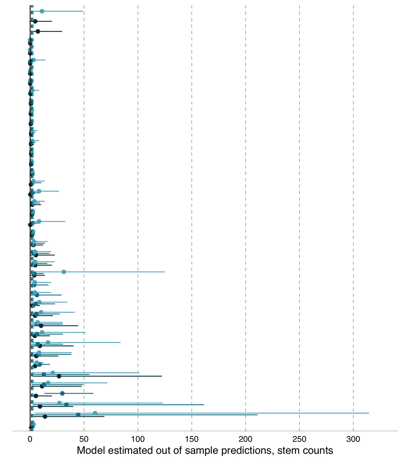
B.1.2.2 Non-truncated \(y_{i}\) meta-analysis forest plot

Below is the non-truncated version of Figure 3.3 showing a forest plot of the out-of-sample predictions, \(y_{i}\), on the response-scale (stem counts), for Eucalyptus analyses, showing the full error bars of all model estimates.

Code

plot_forest_2 <- function(data, intercept = TRUE, MA_mean = TRUE, y_zoom = numeric(2L)){
  if(MA_mean == FALSE){
    data <- filter(data, study_id != "overall")
  }
  
  plot_data <- data %>% 
    group_by(study_id) %>% 
    group_nest() %>% 
    hoist(data, "estimate",.remove = FALSE) %>% 
    hoist(estimate, y50 = 2) %>% 
    select(-estimate) %>% 
    unnest(data) %>% 
    arrange(desc(type)) %>% 
    mutate(type = forcats::as_factor(type)) %>% 
    group_by(type) %>% 
    arrange(desc(y50),.by_group = TRUE) %>% 
    mutate(study_id = forcats::as_factor(study_id),
           point_shape = case_when(str_detect(type, "summary") ~ "diamond",
                                   TRUE ~ "circle"))
  
  p <- ggplot(plot_data, aes(y = estimate, 
                        x =  study_id,
                        ymin = conf.low, 
                        ymax = conf.high,
                        # shape = type,
                        shape = point_shape,
                        colour = estimate_type
                        )) +
    geom_pointrange(position = position_dodge(width = 0.5)) +
    ggforestplot::theme_forest() +
    theme(axis.line = element_line(linewidth = 0.10, colour = "black"),
          axis.line.y = element_blank(),
          text = element_text(family = "Helvetica")) +
    guides(shape = "none", colour = "none") +
    coord_flip(ylim = y_zoom) +
    labs(y = "Model estimated out of sample predictions, stem counts",
         x = element_blank()) +
    scale_y_continuous(breaks = scales::breaks_extended(10)) +
    NatParksPalettes::scale_color_natparks_d("Glacier") 
  
  if(intercept == TRUE){
    p <- p + geom_hline(yintercept = 0)
  }
  
  if(MA_mean == TRUE){
    p <- p +
      geom_hline(aes(yintercept = plot_data %>%
                       filter(type == "summary", estimate_type == "y25") %>%
                       pluck("estimate")),
                 data = data,
                 colour = "#01353D",
                 linetype = "dashed") +
      geom_hline(aes(yintercept = plot_data %>%
                       filter(type == "summary", estimate_type == "y50") %>%
                       pluck("estimate")),
                 data = data,
                 colour = "#088096",
                 linetype = "dashed") +
      geom_hline(aes(yintercept = plot_data %>%
                       filter(type == "summary", estimate_type == "y75") %>%
                       pluck("estimate")),
                 data = data,
                 colour = "#58B3C7" ,
                 linetype = "dashed")
  }
  
  print(p)
}

# ---- new code ----

eucalyptus_yi_plot_data <- 
  ManyEcoEvo_yi_viz %>% 
  filter(dataset == "eucalyptus", model_name == "MA_mod")  %>% 
  unnest(cols = tidy_mod_summary) %>%  
  mutate(response_scale = list(log_back(estimate, std.error, 1000)), 
         .by = c(dataset, estimate_type, term, type), 
         .keep = "used") %>% 
  select(-estimate, -std.error) %>% 
  unnest_wider(response_scale) %>% 
  rename(estimate = mean_origin, conf.low = lower, conf.high = upper) %>% 
  nest(tidy_mod_summary = c(-dataset, -estimate_type)) %>% #extract euc data for plotting (on count scale, not log scale)
  select(dataset, estimate_type, tidy_mod_summary) %>% 
  unnest(cols = tidy_mod_summary) %>% 
  rename(study_id = term) %>% 
  ungroup()

max_x_axis <- 
  eucalyptus_yi_plot_data %>% 
  pluck("conf.high", max) %>% 
  round() + 10

eucalyptus_yi_plot_data %>% 
  plot_forest_2(MA_mean = T, y_zoom = c(0, max_x_axis)) +
  theme(axis.text.y = element_blank())

Figure B.6: Forest plot of meta-analytic estimated out of sample predictions, \(y_{i}\), on the response-scale (stem counts) for *Eucalyptus* analyses. Circles represent individual analysis estimates. Triangles represent the meta-analytic mean for each prediction scenario. Navy blue coloured points correspond to \(y_{25}\) scenario, blue coloured points correspond to the \(y_{50}\) scenario, while light blue points correspond to the \(y_{75}\) scenario. Error bars are 95% confidence intervals. Outliers (i.e. observations with mean estimates more than 3SD above the population parameter mean, see Section B.1.2.1) have been removed prior to model fitting.